Introduction to eBird Status Data Products

Background

The study and conservation of the natural world relies on detailed information about the distributions, abundances, and population trends of species over time. For many taxa, this information is challenging to obtain at relevant geographic scales. The goal of the eBird Status and Trends project is to use data from eBird, the global participatory science bird monitoring program administered by the Cornell Lab of Ornithology, to generate a reliable, standardized source of biodiversity information for the world’s bird populations. To translate the eBird observations into robust data products, we use machine learning to fill spatiotemporal gaps, using local land cover descriptions derived from remote sensing data, while controlling for biases inherent in species observations collected by community scientists. See Fink et al. (2019) for more information about the analysis used to generate these data.

This vignette gives an overview of the eBird Status Data Products, which estimate the full annual cycle distributions, relative abundances, and habitat associations for 2,980 species for the year 2023. For each species, distribution and abundance estimates are available for all 52 weeks of the year across a regular 3 km by 3 km square grid of cells covering the globe. Variation in detectability associated with the search effort is controlled by standardizing the estimates as the expected occurrence rate and count of the species on a 1 hour, 2 km checklist by an expert eBird observer at the optimal time of day and with optimal weather conditions for detecting the species.

Data access

Data access is granted through an Access Request Form at: https://ebird.org/st/request. Filling out this form generates a key to be used with this R package. Our terms of use have been designed to be quite permissive in many cases, particularly academic and research use. When requesting data access, please be sure to carefully read the terms of use and ensure that your intended use is not restricted.

After completing the Access Request Form, you will be provided an eBird Status and Trends Data Products access key, which you will need when downloading data. To store the key so this package can access it when downloading data, use the function set_ebirdst_access_key("XXXXX"), where "XXXXX" is the access key provided to you.

Throughout this vignette, we’ll use a simplified example dataset consisting of estimates for Yellow-bellied Sapsucker in Michigan. This dataset is designed to be small for faster download and, unlike data for other species, is accessible without a key.

library(dplyr)
library(sf)
library(terra)
library(ebirdst)

Downloading data

The data loading functions in this package (those beginning with load_) will download any data they need automatically the first time you use them, so in most cases you don’t need to download data explicitly. For example, calling load_raster("yebsap-example") will download the relative abundance data for the example species if it isn’t already on your computer, then load it into R.

In older versions of ebirdst it was necessary to download data with ebirdst_download_status() before loading it; this is no longer required. However, ebirdst_download_status() is still useful when you want to download all, or a specific subset of, the data products for a species up front rather than one at a time as you load them. The first argument defines the species (as a common name, scientific name, or species code) and the remaining arguments control which data products are downloaded. By default only the most commonly used data products are downloaded, but since this vignette covers all the available data products, we’ll use download_all = TRUE to download everything for the example species now:

# download all data products for the example species
ebirdst_download_status(species = "yebsap-example", download_all = TRUE)

By default, ebirdst_download_status() (and the load_ functions) download data to a centralized directory on your computer. You can see what that directory is with the function ebirdst_data_dir() and you can change the default download directory by setting the environment variable EBIRDST_DATA_DIR, for example by calling usethis::edit_r_environ() and adding a line such as EBIRDST_DATA_DIR=/custom/download/directory/.

IMPORTANT: eBird Status and Trends Data Products are designed to be downloaded and accessed using the ebirdst R package. Data downloaded using this R package have a specific file structure and changing file names or locations will disrupt the ability of functions in this package to access the data. If you prefer to access data for use outside of R, consider downloading data via the eBird Status and Trends website.

Managing downloaded data

Because a new version of the data products is released each year, data for multiple versions can accumulate on disk over time. Use ebirdst_data_inventory() to get a summary of all data currently downloaded, with separate rows for the Status and Trends data products for each species.

ebirdst_data_inventory()
#> eBird Status and Trends data: 135 species, 135 packages (4.3 GB)
#> 
#> 2022 Trends Data Products (9.3 MB)
#>   Brewer's Sparrow (brespa): 3 files, 4.0 MB
#>   Sagebrush Sparrow (sagspa1): 3 files, 2.5 MB
#>   Sage Thrasher (sagthr): 3 files, 2.7 MB
#> 
#> 2023 Status Data Products (4.3 GB)
#>   Acadian Flycatcher (acafly): 2 files, 122.6 KB
#>   American Crow (amecro): 2 files, 248.9 KB
#>   American Goldfinch (amegfi): 2 files, 230.3 KB
#>   American Redstart (amered): 2 files, 247.8 KB
#>   Andean Avocet (andavo1): 3 files, 20.2 MB
#>   Baird's Sparrow (baispa): 6 files, 61.5 MB
#>   Baltimore Oriole (balori): 2 files, 175.9 KB
#>   Band-tailed Earthcreeper (batear1): 2 files, 30.5 MB
#>   Black-and-white Warbler (bawwar): 2 files, 226.8 KB
#>   Buff-browed Foliage-gleaner (bbfgle1): 3 files, 30.2 MB
#>   Black-hooded Sierra Finch (bhsfin1): 3 files, 26.4 MB
#>   Bicolored Hawk (bichaw1): 3 files, 38.7 MB
#>   Black Siskin (blasis1): 3 files, 32.0 MB
#>   Black-bodied Woodpecker (blbwoo3): 3 files, 25.6 MB
#>   Black-headed Duck (blhduc1): 2 files, 22.4 MB
#>   Blue Grosbeak (blugrb1): 2 files, 180.7 KB
#>   Blue Jay (blujay): 2 files, 199.1 KB
#>   Bobolink (boboli): 6 files, 103.5 MB
#>   Brown Thrasher (brnthr): 2 files, 164.3 KB
#>   Broad-winged Hawk (brwhaw): 2 files, 208.7 KB
#>   Bright-rumped Yellow-Finch (bryfin1): 3 files, 29.5 MB
#>   Black-throated Blue Warbler (btbwar): 2 files, 108.1 KB
#>   Black-throated Green Warbler (btnwar): 2 files, 164.0 KB
#>   Blue-crowned Parakeet (bucpar): 3 files, 48.9 MB
#>   Blue-gray Gnatcatcher (buggna): 2 files, 217.1 KB
#>   Blue-headed Vireo (buhvir): 2 files, 181.2 KB
#>   Blue-winged Warbler (buwwar): 2 files, 108.6 KB
#>   Canada Warbler (canwar): 2 files, 149.0 KB
#>   Cedar Waxwing (cedwax): 2 files, 279.0 KB
#>   Cerulean Warbler (cerwar): 2 files, 93.1 KB
#>   Chestnut-collared Longspur (chclon): 6 files, 86.0 MB
#>   Chipping Sparrow (chispa): 2 files, 299.8 KB
#>   Chiloe Wigeon (chiwig1): 28 files, 120.2 MB
#>   Chestnut-sided Warbler (chswar): 2 files, 146.9 KB
#>   Chocolate-vented Tyrant (chvtyr2): 28 files, 110.6 MB
#>   Common Chlorospingus (cobtan1): 3 files, 25.1 MB
#>   Common Potoo (compot1): 28 files, 1.0 GB
#>   Common Yellowthroat (comyel): 2 files, 296.5 KB
#>   Couch's Kingbird (coukin): 2 files, 50.4 KB
#>   Data Coverage (data_coverage): 1 files, 52.9 MB
#>   Dusky-capped Flycatcher (ducfly): 2 files, 141.8 KB
#>   Eastern Bluebird (easblu): 2 files, 179.1 KB
#>   Eastern Phoebe (easpho): 2 files, 183.6 KB
#>   Eastern Towhee (eastow): 2 files, 130.2 KB
#>   Eastern Whip-poor-will (easwpw1): 2 files, 87.3 KB
#>   Eastern Wood-Pewee (eawpew): 2 files, 204.3 KB
#>   Elegant Crested-Tinamou (elctin1): 22 files, 174.6 MB
#>   Field Sparrow (fiespa): 2 files, 148.7 KB
#>   Green-breasted Mango (gnbman): 2 files, 61.8 KB
#>   Golden Eagle (goleag): 5 files, 50.4 MB
#>   Golden-winged Warbler (gowwar): 2 files, 103.1 KB
#>   Groove-billed Ani (grbani): 2 files, 93.0 KB
#>   Great Crested Flycatcher (grcfly): 2 files, 165.0 KB
#>   Greenish Elaenia (greela): 2 files, 196.3 KB
#>   Green Heron (grnher): 2 files, 181.4 KB
#>   Gray Catbird (grycat): 2 files, 209.5 KB
#>   Greenish Yellow-Finch (gryfin3): 3 files, 31.9 MB
#>   Gray Hawk (gryhaw2): 2 files, 57.8 KB
#>   Golden-spotted Ground Dove (gsgdov1): 3 files, 26.2 MB
#>   Gray-breasted Martin (gybmar): 2 files, 293.8 KB
#>   Gray-bellied Shrike-Tyrant (gybsht1): 2 files, 38.9 MB
#>   Straneck's Tyrannulet (gyctyr2): 2 files, 37.1 MB
#>   Hooded Grebe (hoogre1): 2 files, 17.5 MB
#>   Hooded Warbler (hoowar): 2 files, 113.4 KB
#>   Horned Lark (horlar): 2 files, 4.0 MB
#>   Indigo Bunting (indbun): 2 files, 183.1 KB
#>   Kentucky Warbler (kenwar): 2 files, 106.3 KB
#>   Lake Duck (lakduc1): 2 files, 22.5 MB
#>   Least Bittern (leabit): 2 files, 106.6 KB
#>   Least Flycatcher (leafly): 2 files, 221.9 KB
#>   Lesser Nighthawk (lesnig): 2 files, 156.3 KB
#>   Louisiana Waterthrush (louwat): 2 files, 137.7 KB
#>   Magnolia Warbler (magwar): 2 files, 188.8 KB
#>   Mitred Parakeet (mitpar): 3 files, 21.4 MB
#>   Mottle-cheeked Tyrannulet (moctyr2): 3 files, 29.4 MB
#>   Northern Beardless-Tyrannulet (nobtyr): 2 files, 57.5 KB
#>   Northern Parula (norpar): 2 files, 157.1 KB
#>   Northern Waterthrush (norwat): 2 files, 310.3 KB
#>   Northern Rough-winged Swallow (nrwswa): 2 files, 230.1 KB
#>   Orchard Oriole (orcori): 2 files, 171.7 KB
#>   Ovenbird (ovenbi1): 2 files, 192.4 KB
#>   Patagonian Mockingbird (patmoc1): 2 files, 42.6 MB
#>   Patagonian Tinamou (pattin1): 2 files, 21.5 MB
#>   Prairie Warbler (prawar): 2 files, 105.7 KB
#>   Puna Miner (punmin1): 3 files, 25.0 MB
#>   Red-backed Sierra Finch (rbsfin1): 3 files, 20.6 MB
#>   Variable Hawk (rebhaw2): 28 files, 305.8 MB
#>   Red-crested Finch (recfin1): 3 files, 65.2 MB
#>   Red Shoveler (redsho1): 2 files, 26.0 MB
#>   Red-eyed Vireo (reevir1): 2 files, 259.9 KB
#>   Red-fronted Coot (refcoo1): 2 files, 21.4 MB
#>   Red-shouldered Hawk (reshaw): 2 files, 143.0 KB
#>   Rose-breasted Grosbeak (robgro): 2 files, 188.5 KB
#>   Rosy-billed Pochard (robpoc1): 2 files, 27.0 MB
#>   Rose-throated Becard (rotbec): 2 files, 56.8 KB
#>   Ruby-throated Hummingbird (rthhum): 2 files, 164.3 KB
#>   Rufous-chested Dotterel (rucdot1): 28 files, 93.8 MB
#>   Scarlet Tanager (scatan): 2 files, 153.5 KB
#>   Sharp-billed Canastero (shbcan2): 2 files, 39.6 MB
#>   Short-tailed Hawk (shthaw): 2 files, 102.3 KB
#>   Sick's Swift (sicswi1): 3 files, 32.7 MB
#>   Small-billed Elaenia (smbela1): 28 files, 249.7 MB
#>   Song Sparrow (sonspa): 2 files, 278.2 KB
#>   Southern Martin (soumar): 2 files, 24.1 MB
#>   Sprague's Pipit (sprpip): 6 files, 73.7 MB
#>   Summer Tanager (sumtan): 2 files, 174.3 KB
#>   Surf Scoter (sursco): 2 files, 2.4 MB
#>   Swainson's Warbler (swawar): 2 files, 81.0 KB
#>   Tawny-throated Dotterel (tatdot1): 28 files, 128.2 MB
#>   Thick-billed Siskin (thbsis1): 3 files, 24.5 MB
#>   Upland Sandpiper (uplsan): 6 files, 138.5 MB
#>   Vaux's Swift (vauswi): 2 files, 105.4 KB
#>   Warbling Doradito (wardor1): 2 files, 20.7 MB
#>   Western Meadowlark (wesmea): 6 files, 224.1 MB
#>   White-banded Mockingbird (whbmoc1): 2 files, 48.4 MB
#>   White-crested Elaenia (whcela1): 28 files, 185.2 MB
#>   White-eyed Vireo (whevir): 2 files, 123.8 KB
#>   White-throated Flycatcher (whtfly1): 2 files, 57.3 KB
#>   White-tufted Grebe (whtgre3): 2 files, 25.2 MB
#>   Worm-eating Warbler (woewar1): 2 files, 104.5 KB
#>   Wood Thrush (woothr): 2 files, 132.1 KB
#>   Yellow-crowned Night Heron (ycnher): 2 files, 122.7 KB
#>   Yellow-breasted Chat (yebcha): 2 files, 193.4 KB
#>   Yellow-billed Cuckoo (yebcuc): 2 files, 190.4 KB
#>   Yellow-bellied Flycatcher (yebfly): 2 files, 187.9 KB
#>   Yellow-bellied Sapsucker (yebsap): 2 files, 59.5 MB
#>   Yellow-bellied Sapsucker (yebsap-example): 52 files, 9.9 MB
#>   Yellow Cardinal (yelcar1): 2 files, 22.6 MB
#>   Yellow Warbler (yelwar): 2 files, 358.8 KB
#>   Yellow-throated Vireo (yetvir): 2 files, 146.9 KB
#>   Yellow-throated Warbler (yetwar): 2 files, 117.9 KB
#>   Yucatan Nightjar (yucnig1): 2 files, 44.3 KB

To remove data for specific species or version years, use ebirdst_delete(). When called interactively it will display a summary of the data to be removed and ask for confirmation before proceeding. To skip the prompt, use force = TRUE.

# review and confirm before deleting
ebirdst_delete(species = "yebsap-example")

# delete all data for a given version year without prompting
ebirdst_delete(year = 2021, force = TRUE)

Species list

The data frame ebirdst_runs lists all species with eBird Status Data Products available for download.

glimpse(ebirdst_runs)
#> Rows: 2,981
#> Columns: 30
#> $ species_code                   <chr> "yebsap-example", "abetow", "absfin1", …
#> $ scientific_name                <chr> "Sphyrapicus varius", "Melozone aberti"…
#> $ common_name                    <chr> "Yellow-bellied Sapsucker", "Abert's To…
#> $ is_resident                    <lgl> FALSE, TRUE, TRUE, FALSE, TRUE, TRUE, F…
#> $ breeding_quality               <chr> "3", NA, NA, "3", NA, NA, "1", NA, NA, …
#> $ breeding_start                 <date> 2023-05-17, NA, NA, 2023-05-31, NA, NA…
#> $ breeding_end                   <date> 2023-08-16, NA, NA, 2023-08-02, NA, NA…
#> $ nonbreeding_quality            <chr> "3", NA, NA, "3", NA, NA, "1", NA, NA, …
#> $ nonbreeding_start              <date> 2023-11-22, NA, NA, 2023-11-22, NA, NA…
#> $ nonbreeding_end                <date> 2023-03-08, NA, NA, 2023-02-22, NA, NA…
#> $ postbreeding_migration_quality <chr> "3", NA, NA, "3", NA, NA, "0", NA, NA, …
#> $ postbreeding_migration_start   <date> 2023-08-23, NA, NA, 2023-08-09, NA, NA…
#> $ postbreeding_migration_end     <date> 2023-11-15, NA, NA, 2023-11-15, NA, NA…
#> $ prebreeding_migration_quality  <chr> "3", NA, NA, "3", NA, NA, "0", NA, NA, …
#> $ prebreeding_migration_start    <date> 2023-03-15, NA, NA, 2023-03-01, NA, NA…
#> $ prebreeding_migration_end      <date> 2023-05-10, NA, NA, 2023-05-24, NA, NA…
#> $ resident_quality               <chr> NA, "3", "3", NA, "3", "3", NA, "2", "3…
#> $ resident_start                 <date> NA, 2023-01-04, 2023-01-04, NA, 2023-0…
#> $ resident_end                   <date> NA, 2023-12-27, 2023-12-27, NA, 2023-1…
#> $ status_version_year            <dbl> 2023, 2023, 2023, 2023, 2023, 2023, 202…
#> $ has_trends                     <lgl> TRUE, TRUE, FALSE, TRUE, TRUE, FALSE, F…
#> $ trends_season                  <chr> "breeding", "resident", NA, "breeding",…
#> $ trends_region                  <chr> "north_america", "north_america", NA, "…
#> $ trends_start_year              <dbl> 2012, 2012, NA, 2012, 2011, NA, NA, NA,…
#> $ trends_end_year                <dbl> 2022, 2022, NA, 2022, 2021, NA, NA, NA,…
#> $ trends_start_date              <chr> "05-24", "01-25", NA, "05-24", "11-01",…
#> $ trends_end_date                <chr> "08-16", "05-10", NA, "08-02", "05-03",…
#> $ rsquared                       <dbl> 0.8572896, 0.9231821, NA, 0.8570363, 0.…
#> $ beta0                          <dbl> 0.227000849, -0.013923012, NA, 0.689424…
#> $ trends_version_year            <dbl> 2022, 2022, NA, 2022, 2022, NA, NA, NA,…

If you’re working in RStudio, you can use View() to interactively explore this data frame.

All species go through a process of review by an expert on that species prior to being released. The ebirdst_runs data frame contains information from this review process. For migrants, reviewers assess the model estimates for each of the four seasons: breeding, non-breeding, pre-breeding migration, and post-breeding migration. Resident (i.e., non-migratory) species are identified by having TRUE in the is_resident column of ebirdst_runs, and these species are assessed across the whole year rather than seasonally. ebirdst_runs contains two important pieces of information for each season: a quality rating and seasonal dates.

The seasonal dates define the weeks that fall within each season. Breeding and non-breeding season dates are defined for each species as the weeks during those seasons when the species’ population does not move. For this reason, these seasons are also described as stationary periods. Migration periods are defined as the periods of movement between the stationary non-breeding and breeding seasons. Note that for many species these migratory periods include not only movement from breeding grounds to non-breeding grounds, but also post-breeding dispersal, molt migration, and other movements.

Reviewers also examine the model estimates for each season to assess the amount of extrapolation or omission present in the model, and assign an associated quality rating ranging from 0 (lowest quality) to 3 (highest quality). Extrapolation refers to cases where the model predicts occurrence where the species is known to be absent, while omission refers to the model failing to predict occurrence where a species is known to be present.

A rating of 0 implies this season failed review and model results should not be used at all for this period. Ratings of 1-3 correspond to a gradient of more to less extrapolation and/or omission, and we often use a traffic light analogy when referring to them:

1. Red light (1): low quality, extensive extrapolation and/or omission and noise, but at least some regions have estimates that are accurate; can be used with caution in certain regions.
2. Yellow light (2): medium quality, some extrapolation and/or omission; use with caution.
3. Green light (3): high quality, very little or no extrapolation and/or omission; these seasons can be safely used.

Let’s look at the results of the review for our example dataset.

ebirdst_runs |>
  filter(species_code == "yebsap-example") |>
  glimpse()
#> Rows: 1
#> Columns: 30
#> $ species_code                   <chr> "yebsap-example"
#> $ scientific_name                <chr> "Sphyrapicus varius"
#> $ common_name                    <chr> "Yellow-bellied Sapsucker"
#> $ is_resident                    <lgl> FALSE
#> $ breeding_quality               <chr> "3"
#> $ breeding_start                 <date> 2023-05-17
#> $ breeding_end                   <date> 2023-08-16
#> $ nonbreeding_quality            <chr> "3"
#> $ nonbreeding_start              <date> 2023-11-22
#> $ nonbreeding_end                <date> 2023-03-08
#> $ postbreeding_migration_quality <chr> "3"
#> $ postbreeding_migration_start   <date> 2023-08-23
#> $ postbreeding_migration_end     <date> 2023-11-15
#> $ prebreeding_migration_quality  <chr> "3"
#> $ prebreeding_migration_start    <date> 2023-03-15
#> $ prebreeding_migration_end      <date> 2023-05-10
#> $ resident_quality               <chr> NA
#> $ resident_start                 <date> NA
#> $ resident_end                   <date> NA
#> $ status_version_year            <dbl> 2023
#> $ has_trends                     <lgl> TRUE
#> $ trends_season                  <chr> "breeding"
#> $ trends_region                  <chr> "north_america"
#> $ trends_start_year              <dbl> 2012
#> $ trends_end_year                <dbl> 2022
#> $ trends_start_date              <chr> "05-24"
#> $ trends_end_date                <chr> "08-16"
#> $ rsquared                       <dbl> 0.8572896
#> $ beta0                          <dbl> 0.2270008
#> $ trends_version_year            <dbl> 2022

From this, we can see that Yellow-bellied Sapsucker was modeled as a migrant and all four seasons received a quality of 3, the highest rating. Note that there are a variety of trends-specific columns at the end of this data frame that we’ll ignore for now; these columns will be covered in the trends vignette

Data types

For each species, there are a variety of data products available, which can be categorized into the following broad types:

• Weekly raster estimates: weekly estimates of occurrence, count, relative abundance, and proportion of population on a regular grid in GeoTIFF format at three resolutions. These are the core products from which the other products are derived.
• Seasonal raster estimates: seasonal estimates of occurrence, count, relative abundance, and proportion of population on a regular grid in GeoTIFF format at three resolutions. These are derived from the corresponding weekly raster data by summarizing across the weeks falling within each season based on the dates defined in the ebirdst_runs data frame. Only seasons that passed the expert review process are included.
• Seasonal range boundaries: seasonal range boundary polygons in GeoPackage format.
• Regional summary statistics: a variety of summary statistics for countries and states/provinces (e.g. proportion of total population in the region) in CSV format.
• Predictive performance metrics (PPMs): a suite of spatial predictive performance metrics on a regular 27 km by 27 km grid in GeoTIFF format.

Each of these data products will be covered in more detail in the following sections, including details on how to load the data into R. All of the loading functions take a species (given as common name, scientific name, or species code) as their first argument. If the requested data have not already been downloaded, the loading functions will download them automatically on first use, so calling ebirdst_download_status() in advance is optional. If you have used a non-default path argument to ebirdst_download_status() then you will also need to provide the same path argument to the loading functions.

Weekly raster estimates

The core raster data products are the weekly estimates of occurrence, count, and relative abundance. These estimates are derived from an ensemble model producing 100 individual estimates of the expected value of each quantity. The raster data products give the median value across the ensemble for each quantity.

The weekly estimates are all stored in the widely used GeoTIFF raster format, and we refer to them as “weekly cubes” (e.g. the “weekly abundance cube”). All cubes have 52 weeks and cover the entire globe, even for species with ranges only covering a small region. They come with areas of predicted and assumed zeroes. Any cells that are NA represent areas where we didn’t produce model estimates.

All estimates are the ensemble median expected value for a 2 km, 1 hour eBird Traveling Count by an expert eBird observer at the optimal time of day and for optimal weather conditions to observe the given species.

• Occurrence: the expected probability of encountering a species.
• Count: the expected count of a species, conditional on its occurrence at the given location.
• Relative abundance: the expected relative abundance of a species, computed as the product of the probability of occurrence and the count conditional on occurrence. In addition to the median relative abundance, upper and lower confidence intervals (CIs) are provided, defined at the 10th and 90th quantile of relative abundance, respectively.
• Proportion of population: the proportion of the total relative abundance within each cell. This is a derived product calculated by dividing each cell value in the relative abundance raster by the sum of all cell values

All predictions are made on a standard 3 km by 3 km global grid; however, for convenience lower resolution GeoTIFFs are also provided, which are typically much faster to work with. However, note that to keep file sizes small, the example dataset only contains the lowest (27 km) resolution data. The three resolutions are:

• High resolution (3km): the native 3 km resolution data.
• Medium resolution (9km): the 3 km resolution data aggregated by a factor of 3 in each direction resulting in a resolution of 9 km.
• Low resolution (27km): the 3 km resolution data aggregated by a factor of 9 in each direction resulting in a resolution of 27 km.

The function load_raster() is used to load these data into R and takes arguments for product and resolution. The metric argument can also be used to access the relative abundance CIs. All raster products are loaded into R as SpatRaster objects for use with the terra R package. For example,

# weekly, 27km res, median relative abundance
abd_lr <- load_raster(
  "yebsap-example",
  product = "abundance",
  resolution = "27km"
)

# weekly, 27km res, median proportion of population
prop_pop_lr <- load_raster(
  "yebsap-example",
  product = "proportion-population",
  resolution = "27km"
)

# weekly, 27km res, abundance confidence intervals
abd_lower <- load_raster(
  "yebsap-example",
  product = "abundance", metric = "lower",
  resolution = "27km"
)
abd_upper <- load_raster(
  "yebsap-example",
  product = "abundance", metric = "upper",
  resolution = "27km"
)

Each object has 52 layers, one for each week of the year, and layer names store the dates corresponding to the midpoints of each week.

as.Date(names(abd_lr))
#>  [1] "2023-01-04" "2023-01-11" "2023-01-18" "2023-01-25" "2023-02-01"
#>  [6] "2023-02-08" "2023-02-15" "2023-02-22" "2023-03-01" "2023-03-08"
#> [11] "2023-03-15" "2023-03-22" "2023-03-29" "2023-04-05" "2023-04-12"
#> [16] "2023-04-19" "2023-04-26" "2023-05-03" "2023-05-10" "2023-05-17"
#> [21] "2023-05-24" "2023-05-31" "2023-06-07" "2023-06-14" "2023-06-21"
#> [26] "2023-06-28" "2023-07-05" "2023-07-12" "2023-07-19" "2023-07-26"
#> [31] "2023-08-02" "2023-08-09" "2023-08-16" "2023-08-23" "2023-08-30"
#> [36] "2023-09-06" "2023-09-13" "2023-09-20" "2023-09-27" "2023-10-04"
#> [41] "2023-10-11" "2023-10-18" "2023-10-25" "2023-11-01" "2023-11-08"
#> [46] "2023-11-15" "2023-11-22" "2023-11-29" "2023-12-06" "2023-12-13"
#> [51] "2023-12-20" "2023-12-27"

The GeoTIFFs use the Equal Earth coordinate reference system, an equal area projection suitable for global mapping and analysis.

Seasonal raster estimates

The seasonal raster estimates are provided for the same set of products and at the same three resolutions as the weekly estimates. They’re derived from the weekly data by taking the cell-wise mean or max across the weeks within each season. The seasonal boundary dates are defined through a process of expert review of each species, and are available in the data frame ebirdst_runs. Each season is also given a quality score from 0 (fail) to 3 (high quality), and seasons with a score of 0 are not provided.

The function load_raster(period = "seasonal") is used to load these data into R and takes arguments for product, metric and resolution. The data are loaded into R as SpatRaster objects for use with the terra package. For example,

# seasonal, 27km res, mean relative abundance
abd_seasonal_mean <- load_raster(
  "yebsap-example",
  product = "abundance",
  period = "seasonal", metric = "mean",
  resolution = "27km"
)
# season that each layer corresponds to
names(abd_seasonal_mean)
#> [1] "breeding"               "nonbreeding"            "prebreeding_migration" 
#> [4] "postbreeding_migration"
# just the breeding season layer
abd_seasonal_mean[["breeding"]]
#> class       : SpatRaster
#> size        : 618, 1276, 1  (nrow, ncol, nlyr)
#> resolution  : 27000, 27000  (x, y)
#> extent      : -1.7226e+07, 1.7226e+07, -8343000, 8343000  (xmin, xmax, ymin, ymax)
#> coord. ref. : WGS 84 / Equal Earth Greenwich (EPSG:8857)
#> source      : yebsap-example_abundance_seasonal_mean_27km_2023.tif
#> name        : breeding
#> min value   :        0
#> max value   : 1.021968

# seasonal, 27km res, max occurrence
occ_seasonal_max <- load_raster(
  "yebsap-example",
  product = "occurrence",
  period = "seasonal", metric = "max",
  resolution = "27km"
)

Finally, as a convenience, the data products include year-round rasters summarizing the mean or max across all weeks that fall within a season that passed the expert review process. These can be accessed similarly to the seasonal products, but with period = "full-year" instead. For example, these layers can be used in conservation planning to assess the most important sites across the full range and full annual cycle of a species.

# full year, 27km res, maximum relative abundance
abd_fy_max <- load_raster(
  "yebsap-example",
  product = "abundance",
  period = "full-year", metric = "max",
  resolution = "27km"
)

Range boundaries

Seasonal range polygons are defined as the boundaries of non-zero seasonal relative abundance estimates, which are then (optionally) smoothed to produce more aesthetically pleasing polygons using the smoothr package. They are provided in the widely used GeoPackage format and can be loaded into R with load_ranges(), which returns a set of spatial features for use with the sf R package. By default the smoothed ranges are returned, but using smoothed = FALSE will return the raw, unsmoothed range polygons. Note that only low and medium resolution ranges are provided. For example:

# seasonal, 27km res, smoothed ranges
ranges <- load_ranges("yebsap-example", resolution = "27km")
ranges
#> Simple feature collection with 4 features and 8 fields
#> Geometry type: MULTIPOLYGON
#> Dimension:     XY
#> Bounding box:  xmin: -90.41254 ymin: 41.69681 xmax: -82.4146 ymax: 48.19076
#> Geodetic CRS:  WGS 84
#> # A tibble: 4 × 9
#>   species_code scientific_name    common_name       prediction_year type  season
#>   <chr>        <chr>              <chr>                       <int> <chr> <chr> 
#> 1 yebsap       Sphyrapicus varius Yellow-bellied S…            2023 range breed…
#> 2 yebsap       Sphyrapicus varius Yellow-bellied S…            2023 range nonbr…
#> 3 yebsap       Sphyrapicus varius Yellow-bellied S…            2023 range postb…
#> 4 yebsap       Sphyrapicus varius Yellow-bellied S…            2023 range prebr…
#> # ℹ 3 more variables: start_date <date>, end_date <date>,
#> #   geom <MULTIPOLYGON [°]>

# subset to just the breeding season range using dplyr
range_breeding <- filter(ranges, season == "breeding")

Regional summary statistics

Regional summaries of the seasonal raster estimates are also provided for a standard set of regions (countries and states/provinces). These summary statistics can be loaded with load_regional_stats():

regional <- load_regional_stats("yebsap-example")
glimpse(regional)
#> Rows: 8
#> Columns: 15
#> $ species_code           <chr> "yebsap-example", "yebsap-example", "yebsap-exa…
#> $ region_type            <chr> "country", "country", "country", "country", "st…
#> $ region_code            <chr> "USA", "USA", "USA", "USA", "USA-MI", "USA-MI",…
#> $ region_name            <chr> "United States", "United States", "United State…
#> $ continent_code         <chr> "NA", "NA", "NA", "NA", "NA", "NA", "NA", "NA"
#> $ continent_name         <chr> "North America", "North America", "North Americ…
#> $ season                 <chr> "breeding", "nonbreeding", "postbreeding_migrat…
#> $ abundance_mean         <dbl> 0.114652605, 0.123534772, 0.073477334, 0.084178…
#> $ total_pop_percent      <dbl> 0.3034155366, 0.9497140025, 0.7885750146, 0.435…
#> $ continent_pop_percent  <dbl> 0.3034155366, 0.9497140025, 0.7885750146, 0.435…
#> $ range_occupied_percent <dbl> 0.25990556, 0.40518814, 0.54434548, 0.49810429,…
#> $ range_total_percent    <dbl> 0.231714761, 0.801986186, 0.720437099, 0.573623…
#> $ range_days_occupation  <int> 98, 112, 91, 63, 98, 112, 91, 49
#> $ max_week               <chr> "2023-08-16", "2023-11-22", "2023-10-18", "2023…
#> $ max_week_percent_pop   <dbl> 0.4100934563, 0.9638256049, 0.9979910064, 0.985…

The eight summary statistics are defined as:

• abundance_mean: mean relative abundance in the region.
• total_pop_percent: the proportion of the seasonal modeled population within the region.
• continent_pop_percent: the proportion of the seasonal modeled population for the continent within the region. The continent_name column identifies the continent that the region falls within. Note that Yellow-bellied Sapsucker only occurs in North America so the total and continental proportions are identical.
• range_occupied_percent: the proportion of the region occupied by the species during the given season.
• range_total_percent: the proportion of the species seasonal range falling within the region.
• range_days_occupation: number of days of the season that the region was occupied by this species.
• max_week: the week of the year with the highest proportion of the modeled population falling within the region.
• max_week_percent_pop: the proportion of the modeled population within the region in max_week, i.e. the maximum weekly value.

Regional statistics for all species

The regional summary statistics described above are also compiled into a single dataset covering all species with eBird Status Data Products, rather than being split across the individual species data packages. This dataset can be accessed with ebirdst_regional_stats(), which downloads the file on first use and loads it in a single step. Subsequent calls load the already downloaded file directly. As with the load_*() functions, the download happens automatically without prompting.

As an example, we can use this dataset to get a list of all species with breeding or resident season estimates in a given region, e.g. Taiwan. We subset to the region and seasons of interest, keep just the species code, season, and proportion of the population columns, then join to ebirdst_runs to attach the common and scientific names:

# download (on first use) and load regional stats for all species
regional_all <- ebirdst_regional_stats()

# breeding and resident species in taiwan
taiwan <- regional_all |>
  filter(
    region_name == "Taiwan",
    season %in% c("breeding", "resident")
  ) |>
  select(species_code, season, total_pop_percent)

# join to ebirdst_runs to attach common and scientific names
taiwan <- taiwan |>
  inner_join(ebirdst_runs, by = "species_code") |>
  arrange(desc(total_pop_percent)) |>
  select(species_code, common_name, scientific_name, season, total_pop_percent)
taiwan

Predictive performance metrics (PPMs)

A subset of 10% of the eBird observations is excluded from model training to be used as a test set. For each submodel making up the eBird Status model ensemble, model predictions are compared to actual occurrence and count for a spatiotemporally subsampled version of the test dataset to generate a suite of predictive performance metrics (PPMs) at the base model level. These PPMs are then summarized across the ensemble to a 27 km resolution raster grid, where the cell values are the average across all models in the ensemble contributing to that cell. For migrants, PPMs are provided at weekly temporal resolution, in the form of a stack of 52 rasters for each metric, while for residents, year round PPMs are provided in the form of a single raster for each metric.

In total, nineteen predictive performance metrics are provided in four categories. Binary PPMs compare the predicted presence/absence to observed detection/non-detection for all test checklists.

• binary_f1: F1-score.
• binary_mcc: Matthews Correlation Coefficient (MCC).
• binary_prevalence: the observed detection probability after spatiotemporal subsampling.

Occurrence PPMs compare the predicted encounter rate with the observed detection/non-detection for the subset of test checklists within the predicted range boundary.

• occ_bernoulli_dev: the proportion of the Bernoulli deviance explained.
• occ_bin_spearman: test observations are binned by predicted encounter rate with bin widths of 0.05, then the mean observed prevalence and predicted encounter rate are calculated within bins. This metric is the Spearman’s rank correlation coefficient comparing the observed and predicted binned mean values.
• occ_brier: Brier score, i.e. the mean squared difference between predicted encounter rate and observed detection/non-detection.
• occ_pr_auc: area on the precision-recall curve (PR-AUC)
• occ_pr_auc_gt_prev: the proportion of the ensemble for which the PR-AUC is greater than observed prevalence, which indicates that the model is performing better than random guessing.
• occ_pr_auc_normalized: the PR-AUC normalized to account for class imbalance so that a value of 0 represents performance equal to random guessing and a value of 1 represents perfect classification.

Count PPMs compare the predicted count with the observed count for the subset of test checklists within the predicted range boundary and where the species was detected.

• count_log_pearson: the Pearson correlation coefficient comparing the logarithm of the predicted count with the logarithm of the observed count.
• count_mae: mean absolute error (MAE).
• count_poisson_dev: the proportion of the Poisson deviance explained.
• count_rmse: root mean squared error (RMSE).
• count_spearman: Spearman’s rank correlation coefficient.

Abundance PPMs compare the predicted relative abundance with the observed count for the full set of tests checklists.

• abd_log_pearson: Pearson correlation coefficient comparing the logarithm of the predicted relative abundance with the logarithm of the observed count.
• abd_mae: the mean absolute error (MAE).
• abd_poisson_dev: the proportion of the Poisson deviance explained.
• abd_rmse: root mean squared error (RMSE).
• abd_spearman: Spearman’s rank correlation coefficient.

The spatial PPMs can be loaded using load_ppm(). For example, to load the normalized PR-AUC for the example dataset use:

pr_auc <- load_ppm("yebsap-example", ppm = "occ_pr_auc_normalized")
print(pr_auc)
#> class       : SpatRaster
#> size        : 618, 1276, 52  (nrow, ncol, nlyr)
#> resolution  : 27000, 27000  (x, y)
#> extent      : -1.7226e+07, 1.7226e+07, -8343000, 8343000  (xmin, xmax, ymin, ymax)
#> coord. ref. : WGS 84 / Equal Earth Greenwich (EPSG:8857)
#> source      : yebsap-example_ppm_occ-pr-auc-normalized_mean_27km_2023.tif
#> names       :    01-04,    01-11,    01-18,    01-25,    02-01,    02-08, ...
#> min values  : 0.111343, 0.098129, 0.018913, 0.018913, 0.018913, 0.014034, ...
#> max values  : 0.734387, 0.734387, 0.796934, 0.796934,        1,        1, ...

Since Yellow-bellied Sapsucker is a migrant, there are 52 layers, one for each week of the year, giving the mean PR-AUC for each 27 km by 27 km grid cell. We can produce a simple plot of PR-AUC for a week in the middle of the year. Note that trim() is used to trim the global raster down to just show the area with data (the state of Michigan in this example dataset).

plot(trim(pr_auc[[26]]))

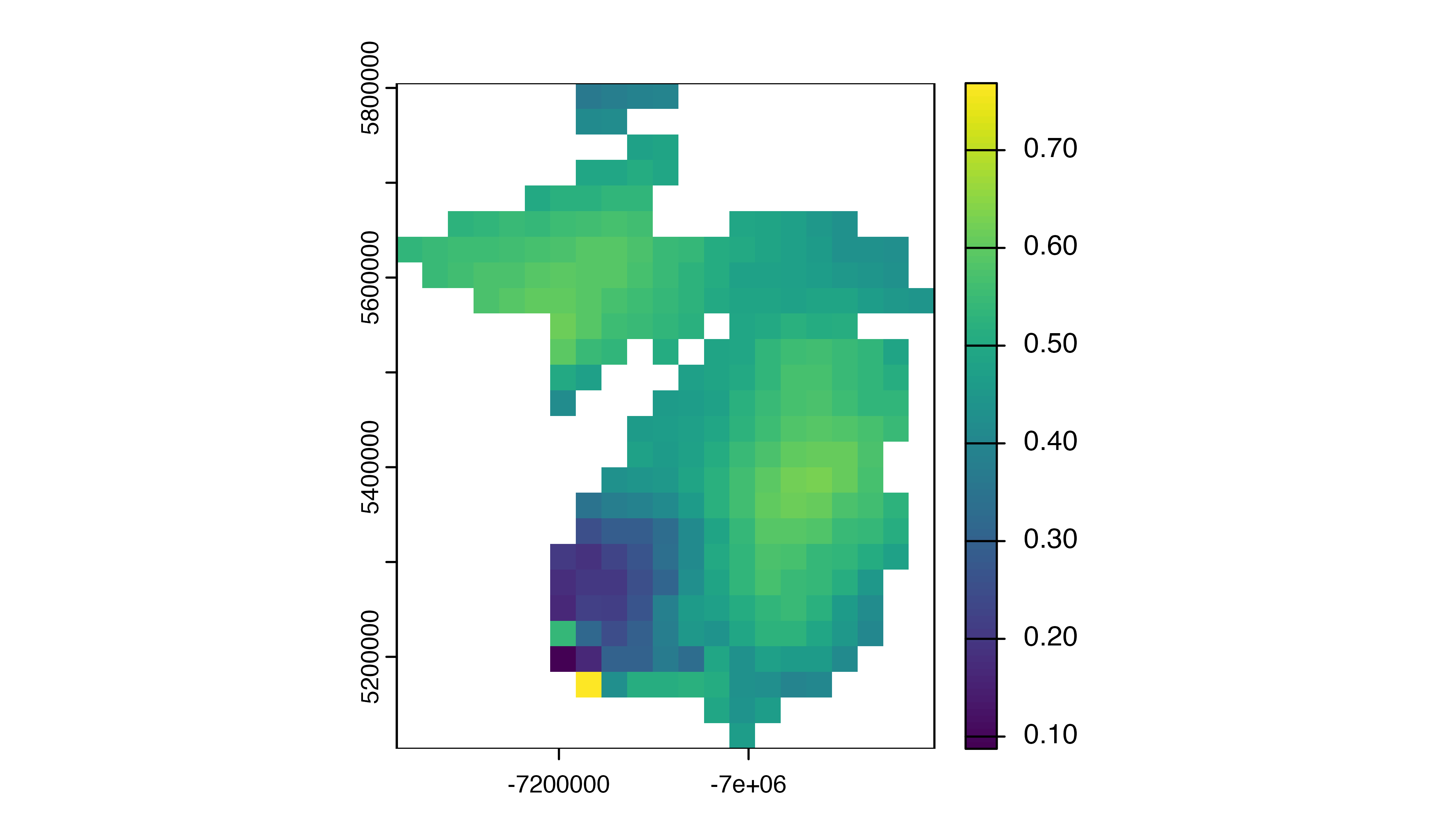
See the applications vignette for a more detailed example of how to use the PPMs.

Data coverage

In addition to the species-specific data products discussed above, ebirdst provides access to two species-agnostic data products from our data coverage workflow. The data products in GeoTIFF format provide weekly estimates on a regular 3 km by 3 km grid of

1. Site selection probability: the modeled probability (0-1) that a grid cell of a certain habitat configuration received an eBird checklist within that region and season.
2. Spatial coverage: the fraction (0-1) of grid cells within that region and season that checklists for the given week.

These data products identify areas where the coverage of eBird data is relatively high or low, which can be used to prioritize areas for increased data collection. For example, to load and map the site selection probability for the week of May 10, use load_data_coverage(), which will download the requested weeks automatically if they haven’t already been downloaded. If you prefer to download the data coverage products in advance, use ebirdst_download_data_coverage().

site_sel <- load_data_coverage("selection-probability", weeks = "05-10")
plot(site_sel, axes = FALSE)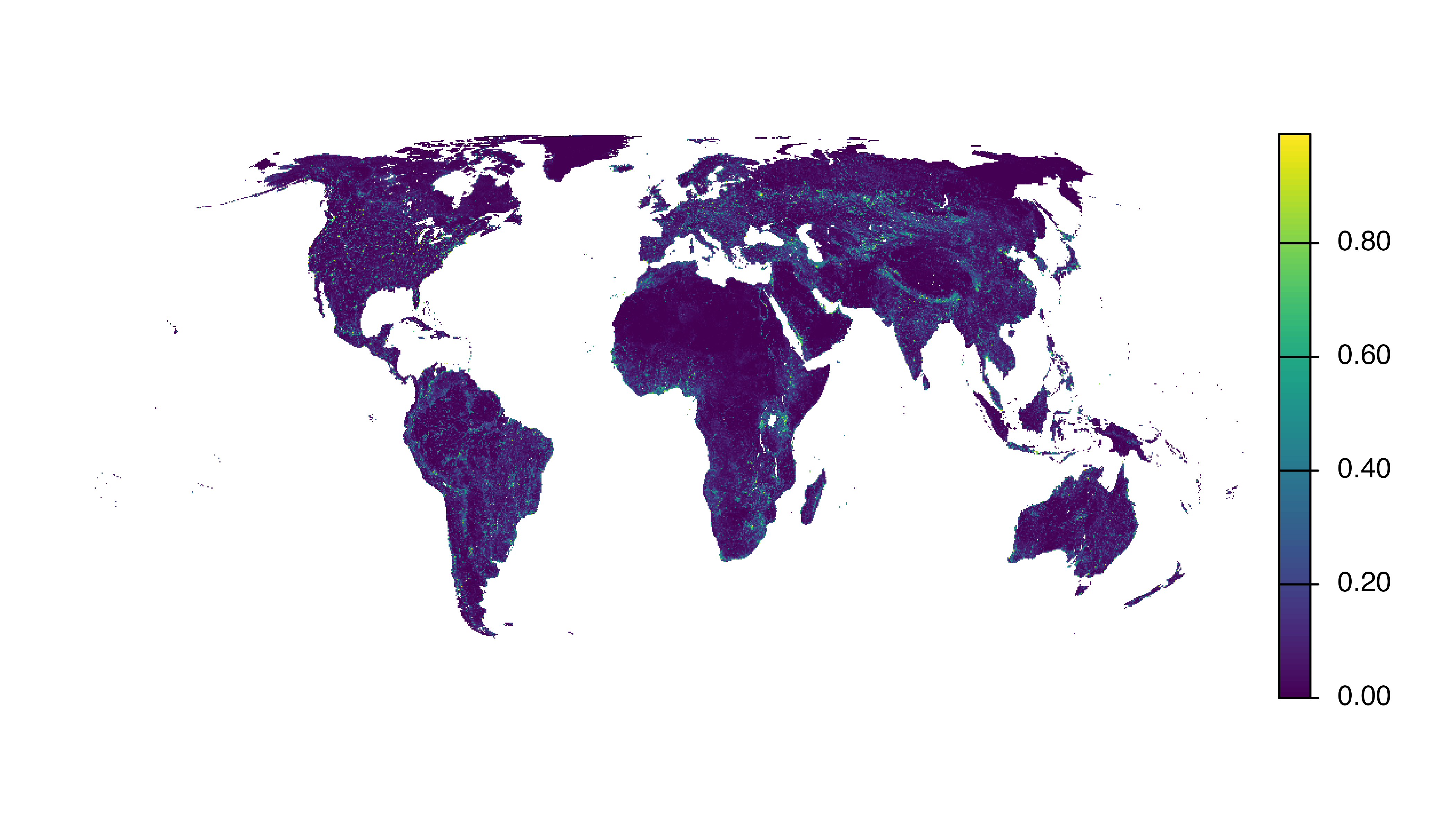

References

Fink, D., T. Auer, A. Johnston, V. Ruiz‐Gutierrez, W.M. Hochachka, S. Kelling. 2019. Modeling avian full annual cycle distribution and population trends with citizen science data. Ecological Applications, 00(00):e02056. doi: 10.1002/eap.2056