library(auk)
library(dplyr)
library(ggplot2)
library(gridExtra)
library(lubridate)
library(readr)
library(sf)

f_sed <- "data-raw/ebd_US-GA_woothr_smp_relOct-2023_sampling.txt"
checklists <- read_sampling(f_sed)
glimpse(checklists)
#> Rows: 1,120,132
#> Columns: 31
#> $ checklist_id              <chr> "S78945522", "S100039674", "S7892023", "S789…
#> $ last_edited_date          <chr> "2021-04-13 15:28:08.442812", "2022-01-03 14…
#> $ country                   <chr> "United States", "United States", "United St…
#> $ country_code              <chr> "US", "US", "US", "US", "US", "US", "US", "U…
#> $ state                     <chr> "Georgia", "Georgia", "Georgia", "Georgia", …
#> $ state_code                <chr> "US-GA", "US-GA", "US-GA", "US-GA", "US-GA",…
#> $ county                    <chr> "Monroe", "Monroe", "Chatham", "Chatham", "C…
#> $ county_code               <chr> "US-GA-207", "US-GA-207", "US-GA-051", "US-G…
#> $ iba_code                  <chr> NA, NA, NA, NA, NA, NA, NA, NA, NA, NA, NA, …
#> $ bcr_code                  <int> 29, 29, NA, NA, NA, NA, NA, NA, NA, NA, NA, …
#> $ usfws_code                <chr> NA, NA, NA, NA, NA, NA, NA, NA, NA, NA, NA, …
#> $ atlas_block               <chr> NA, NA, NA, NA, NA, NA, NA, NA, NA, NA, NA, …
#> $ locality                  <chr> "Rum Creek M.A.R.S.H. Project", "Rum Creek M…
#> $ locality_id               <chr> "L876993", "L876993", "L877616", "L877614", …
#> $ locality_type             <chr> "H", "H", "H", "H", "H", "H", "H", "H", "H",…
#> $ latitude                  <dbl> 33.1, 33.1, 31.4, 31.7, 31.7, 31.7, 31.7, 31…
#> $ longitude                 <dbl> -83.9, -83.9, -80.2, -80.4, -80.4, -80.4, -8…
#> $ observation_date          <date> 1997-12-31, 1997-02-23, 1983-09-13, 1984-02…
#> $ time_observations_started <chr> NA, NA, NA, NA, NA, NA, NA, "07:20:00", "15:…
#> $ observer_id               <chr> "obs1675368", "obs198993", "obs243631", "obs…
#> $ sampling_event_identifier <chr> "S78945522", "S100039674", "S7892023", "S789…
#> $ protocol_type             <chr> "Historical", "Historical", "Incidental", "I…
#> $ protocol_code             <chr> "P62", "P62", "P20", "P20", "P20", "P20", "P…
#> $ project_code              <chr> "EBIRD", "EBIRD", "EBIRD", "EBIRD", "EBIRD",…
#> $ duration_minutes          <int> NA, NA, NA, NA, NA, NA, NA, 400, 120, NA, NA…
#> $ effort_distance_km        <dbl> NA, NA, NA, NA, NA, NA, NA, 64.4, 40.2, NA, …
#> $ effort_area_ha            <dbl> NA, NA, NA, NA, NA, NA, NA, NA, NA, NA, NA, …
#> $ number_observers          <int> 1, NA, NA, NA, NA, NA, NA, 5, 15, NA, NA, NA…
#> $ all_species_reported      <lgl> TRUE, TRUE, FALSE, FALSE, FALSE, FALSE, FALS…
#> $ group_identifier          <chr> NA, NA, NA, NA, NA, NA, NA, NA, NA, NA, NA, …
#> $ trip_comments <chr> NA, NA, "Joel McNeal entering accepted recor…2 eBird Data
2.1 Introduction
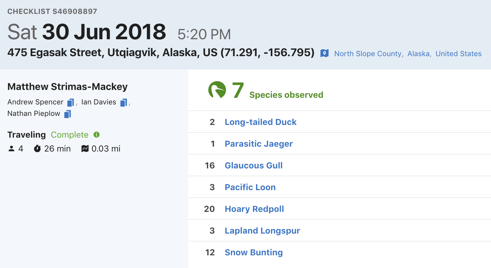
eBird data are collected and organized around the concept of a checklist, representing observations from a single birding event, such as a 1 km walk through a park or 15 minutes observing bird feeders in your backyard. Each checklist contains a list of species observed, counts of the number of individuals seen of each species, the location and time of the observations, information on the type of survey performed, and measures of the effort expended while collecting these data. The following image depicts a typical eBird checklist as viewed on the eBird website:
There are three key characteristics that distinguish eBird from many other citizen science projects and facilitate robust ecological analyses. First, observers specify the survey protocol they used, whether it’s traveling, stationary, incidental (i.e., if the observations were collected when birding was not the primary activity), or one of the other protocols. These protocols are designed to be flexible, allowing observers to collect data during their typical birding outings. Second, in addition to typical information on when and where the observations were made, observers record effort information specifying how long they searched, how far they traveled, and the total number of observers in their party. Collecting this data facilitates robust analyses by allowing researchers to account for variation in the observation process (La Sorte et al. 2018; Kelling et al. 2018). Finally, observers are asked to indicate whether they are reporting all the birds they were able to detect and identify. Checklists with all species reported, known as complete checklists, enable researchers to infer counts of zero individuals for the species that were not reported. If checklists are not complete, it’s not possible to ascertain whether the absence of a species on a list was a non-detection or the result of a participant not recording the species.
Citizen science projects occur on a spectrum from those with predefined sampling structures that resemble more traditional survey designs (such as the Breeding Bird Survey in the United States), to those that are unstructured and collect observations opportunistically (such as iNaturalist). We refer to eBird as a semi-structured project (Kelling et al. 2018), having flexible, easy to follow protocols that attract many participants, but also collecting data on the observation process and allowing non-detections to be inferred on complete checklists.
In this chapter, we’ll highlight some of the challenges associated with using eBird data. Then we’ll demonstrate how to download eBird data for a given region and species. Next, we’ll show how to import the data into R, apply filters to it, and use complete checklists to produce detection/non-detection data suitable for modeling species distribution and abundance. Finally, we’ll perform some pre-processing steps required to ensure proper analysis of the data.
TipTip
We use the terms detection and non-detection rather than the more common terms presence and absence throughout this guide to reflect the fact that an inferred count of zero does not necessarily mean that a species is absent, only that it was not detected on the checklist in question.
2.2 Challenges associated with eBird data
Despite the strengths of eBird data, species observations collected through citizen science projects present a number of challenges that are not found in conventional scientific data. The following are some of the primary challenges associated with these data; challenges that will be addressed throughout this guide:
- Taxonomic bias: participants often have preferences for certain species, which may lead to preferential recording of some species over others (Greenwood 2007; Tulloch and Szabo 2012). Restricting analyses to complete checklists largely mitigates this issue.
- Spatial bias: most participants in citizen science surveys sample near their homes (Luck et al. 2004), in easily accessible areas such as roadsides (Kadmon, Farber, and Danin 2004), or in areas and habitats of known high biodiversity (Prendergast et al. 1993). A simple method to reduce the spatial bias that we describe is to create an equal area grid over the region of interest, and sample a given number of checklists from within each grid cell.
- Temporal bias: participants preferentially sample when they are available, such as weekends (Courter et al. 2013), and at times of year when they expect to observe more birds, notably in the United States there is a large increase in eBird submissions during spring migration (Sullivan et al. 2014). Furthermore, eBird has steadily increased in popularity over time, leading a strong bias towards more data in recent years. To address the weekend bias, we recommend using a temporal scale of a week or multiple weeks for most analyses. Temporal biases at longer time scales can be addressed by subsampling the data to produce a more even temporal distribution.
- Class imbalance: bird species that are rare or hard to detect may have data with high class imbalance, with many more checklists with non-detections than detections. For these species, a distribution model predicting that the species is absent everywhere will have high accuracy, but no ecological value. We’ll follow the methods for addressing class imbalance proposed by Robinson et al. (2018), sampling the data to artificially increase the prevalence of detections prior to modeling.
- Spatial precision: the spatial location of an eBird checklist is given as a single latitude-longitude point; however, this may not be precise for two main reasons. First, for traveling checklists, this location represents just one point on the journey. Second, eBird checklists are often assigned to a hotspot (a common location for all birders visiting a popular birding site) rather than their true location. For these reasons, it’s not appropriate to align the eBird locations with very precise habitat variables, and we recommend summarizing variables within a neighborhood around the checklist location.
- Variation in detectability/effort: detectability describes the probability of a species that is present in an area being detected and identified. Detectability varies by season, habitat, and species (Johnston et al. 2014, 2018). Furthermore, eBird data are collected with high variation in effort, time of day, number of observers, and external conditions such as weather, all of which can affect the detectability of species (Ellis and Taylor 2018; Oliveira et al. 2018). Therefore, detectability is particularly important to consider when comparing between seasons, habitats or species. Since eBird uses a semi-structured protocol, that collects data on the observation process, we’ll be able to account for a larger proportion of this variation in our analyses.
The remainder of this guide will demonstrate how to address these challenges using real data from eBird to produce reliable estimates of species distributions. In general, we’ll take a two-pronged approach to dealing with unstructured data and maximizing the value of citizen science data: imposing more structure onto the data via data filtering and including predictor variables describing the observation process in our models to account for the remaining variation.
2.3 Downloading data
eBird data are typically distributed in two parts: observation data and checklist data. In the observation dataset, each row corresponds to the sighting of a single species on a checklist, including the count and any other species-level information (e.g. age, sex, species comments, etc.). In the checklist dataset, each row corresponds to a checklist, including the date, time, location, effort (e.g. distance traveled, time spent, etc.), and any additional checklist-level information (e.g. whether this is a complete checklist or not). The two datasets can be joined together using a unique checklist identifier (sometimes referred to as the sampling event identifier).
The observation and checklist data are released as tab-separated text files referred to as the eBird Basic Dataset (EBD) and the Sampling Event Data (SED), respectively. These files are released monthly and contain all validated bird sightings in the eBird database at the time of release. Both of these datasets can be downloaded in their entirety or a subset for a given species, region, or time period can be requested via the Custom Download form. We strongly recommend against attempting to download the complete EBD since it’s well over 100GB at the time of writing. Instead, we will demonstrate a workflow using the Custom Download approach. In what follows, we will assume you have followed the instructions for requesting access to eBird data outlined in the previous chapter.

In the interest of making examples concrete, throughout this guide, we’ll focus on moedeling the distribution of Wood Thrush in Georgia (the US state, not the country) in June. Wood Thrush breed in deciduous forests of the eastern United States. We’ll start by downloading the corresponding eBird observation (EBD) and checklist (SED) data by visiting the eBird Basic Dataset download page and filling out the Custom Download form to request Wood Thrush observations from Georgia. Make sure you check the box “Include sampling event data”, which will include the SED in the data download in addition to the EBD.

Once the data are ready, you will receive an email with a download link. The downloaded data will be in a compressed .zip format, and should be unarchived. The resulting directory will contain a two text files: one for the EBD (e.g. ebd_US-GA_woothr_smp_relOct-2023.txt) containing all the Wood Thrush observations from Georgia and one for the SED (e.g. ebd_US-GA_woothr_smp_relOct-2023_sampling.txt) containing all checklists from Georgia. The relOct-2023 component of the file name describes which version of the EBD this dataset came from; in this case it’s the October 2023 release.
TipTip
Since the EBD is updated monthly, you will likely receive a different version of the data than the October 2023 version used throughout the rest of this lesson. Provided you update the filenames of the downloaded files accordingly, the difference in versions will not be an issue. However, if you want to download and use exactly the same files used in this lesson, you can download the corresponding EBD zip file.
2.4 Importing eBird data into R
The previous step left us with two tab separated text files, one for the EBD (i.e. observation data) and one for the SED (i.e. checklist data). For this example, we’ve placed the downloaded text files in the data-raw/ sub-directory of our working directory. Feel free to put these files in a place that’s convenient to you, but make sure to update the file paths in the following code blocks.
The auk functions read_ebd() or read_sampling() are designed to import the EBD and SED, respectively, into R. First let’s import the checklist data (SED).
ImportantCheckpoint
Take some time to explore the variables in the checklist dataset. If you’re unsure about any of the variables, consult the metadata document that came with the data download (eBird_Basic_Dataset_Metadata_v1.15.pdf).
For some applications, only the checklist data are required. For example, the checklist data can be used to investigate the spatial and temporal distribution of eBird data within a region. This dataset can also be used to explore how much variation there is in the effort variables and identify checklists that have low spatial or temporal precision.
NoteSolution
More than 95% of checklists are less than 10 km in length; however, some checklists are as long as 80 km in length. Long traveling checklists have lower spatial precision so they should generally be removed prior to analysis.
checklists_traveling <- filter(checklists, protocol_type == "Traveling")
ggplot(checklists_traveling) +
  aes(x = effort_distance_km) +
  geom_histogram(binwidth = 1,
                 aes(y = after_stat(count / sum(count)))) +
  scale_y_continuous(limits = c(0, NA), labels = scales::label_percent()) +
  labs(x = "Distance traveled [km]",
       y = "% of eBird checklists",
       title = "Distribution of distance traveled on eBird checklists")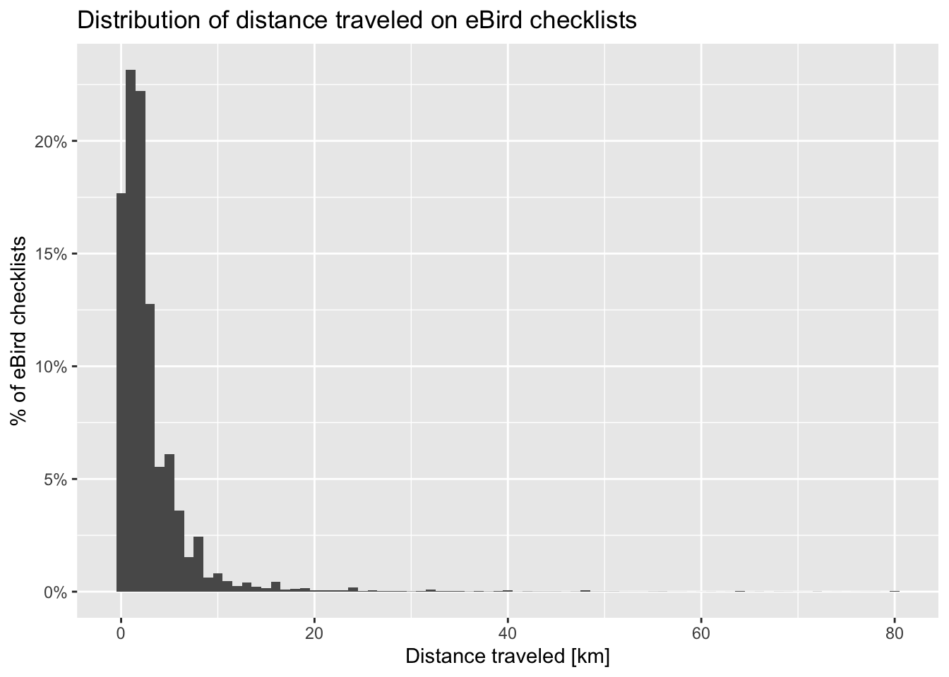
Now let’s import the observation data.
f_ebd <- "data-raw/ebd_US-GA_woothr_smp_relOct-2023.txt"
observations <- read_ebd(f_ebd)
glimpse(observations)
#> Rows: 41,432
#> Columns: 48
#> $ checklist_id              <chr> "G10000432", "G10001259", "G10002209", "G100…
#> $ global_unique_identifier  <chr> "URN:CornellLabOfOrnithology:EBIRD:OBS168581…
#> $ last_edited_date          <chr> "2023-04-16 08:18:20.744008", "2023-05-08 08…
#> $ taxonomic_order           <dbl> 28347, 28347, 28347, 28347, 28347, 28347, 28…
#> $ category                  <chr> "species", "species", "species", "species", …
#> $ taxon_concept_id          <chr> "avibase-8E1D9327", "avibase-8E1D9327", "avi…
#> $ common_name               <chr> "Wood Thrush", "Wood Thrush", "Wood Thrush",…
#> $ scientific_name           <chr> "Hylocichla mustelina", "Hylocichla mustelin…
#> $ exotic_code               <chr> NA, NA, NA, NA, NA, NA, NA, NA, NA, NA, NA, …
#> $ observation_count         <chr> "1", "2", "2", "2", "4", "1", "1", "2", "1",…
#> $ breeding_code             <chr> NA, NA, NA, NA, NA, NA, NA, NA, NA, NA, NA, …
#> $ breeding_category         <chr> NA, NA, NA, NA, NA, NA, NA, NA, NA, NA, NA, …
#> $ behavior_code             <chr> NA, NA, NA, NA, NA, NA, NA, NA, NA, NA, NA, …
#> $ age_sex                   <chr> NA, NA, NA, NA, NA, NA, NA, NA, NA, NA, NA, …
#> $ country                   <chr> "United States", "United States", "United St…
#> $ country_code              <chr> "US", "US", "US", "US", "US", "US", "US", "U…
#> $ state                     <chr> "Georgia", "Georgia", "Georgia", "Georgia", …
#> $ state_code                <chr> "US-GA", "US-GA", "US-GA", "US-GA", "US-GA",…
#> $ county                    <chr> "Bibb", "Laurens", "Wilkes", "Bartow", "Jasp…
#> $ county_code               <chr> "US-GA-021", "US-GA-175", "US-GA-317", "US-G…
#> $ iba_code                  <chr> NA, NA, NA, NA, "US-GA_3108", NA, NA, NA, NA…
#> $ bcr_code                  <int> 27, 27, 29, 28, 29, 29, 29, 29, 29, 29, 29, …
#> $ usfws_code                <chr> NA, NA, NA, NA, "USFWS_315", NA, NA, NA, NA,…
#> $ atlas_block               <chr> NA, NA, NA, NA, NA, NA, NA, NA, NA, NA, NA, …
#> $ locality                  <chr> "Bondsview Rd., Macon", "Wendell Dixon Rd. D…
#> $ locality_id               <chr> "L1286522", "L19345770", "L23606711", "L1118…
#> $ locality_type             <chr> "H", "P", "P", "H", "H", "H", "H", "H", "H",…
#> $ latitude                  <dbl> 32.8, 32.7, 33.8, 34.2, 33.1, 33.9, 33.8, 33…
#> $ longitude                 <dbl> -83.6, -83.0, -82.8, -84.7, -83.8, -83.2, -8…
#> $ observation_date          <date> 2023-04-15, 2023-04-15, 2023-04-15, 2023-04…
#> $ time_observations_started <chr> "08:18:00", "10:00:00", "09:11:00", "08:00:0…
#> $ observer_id               <chr> "obsr139202,obsr617813,obsr198476,obsr267268…
#> $ sampling_event_identifier <chr> "S133806681,S133806682,S133857533,S133858448…
#> $ protocol_type             <chr> "Traveling", "Traveling", "Traveling", "Trav…
#> $ protocol_code             <chr> "P22", "P22", "P22", "P22", "P22", "P22", "P…
#> $ project_code              <chr> "EBIRD", "EBIRD", "EBIRD", "EBIRD", "EBIRD",…
#> $ duration_minutes          <int> 57, 45, 102, 287, 170, 99, 85, 71, 32, 10, 4…
#> $ effort_distance_km        <dbl> 2.849, 9.656, 8.005, 5.404, 11.955, 5.501, 2…
#> $ effort_area_ha            <dbl> NA, NA, NA, NA, NA, NA, NA, NA, NA, NA, NA, …
#> $ number_observers          <int> 11, 2, 3, 12, 2, 3, 2, 2, 1, 1, 2, 2, 2, 2, …
#> $ all_species_reported      <lgl> TRUE, TRUE, TRUE, TRUE, TRUE, TRUE, TRUE, TR…
#> $ group_identifier          <chr> "G10000432", "G10001259", "G10002209", "G100…
#> $ has_media                 <lgl> FALSE, FALSE, FALSE, FALSE, FALSE, FALSE, FA…
#> $ approved                  <lgl> TRUE, TRUE, TRUE, TRUE, TRUE, TRUE, TRUE, TR…
#> $ reviewed                  <lgl> FALSE, FALSE, FALSE, FALSE, FALSE, FALSE, FA…
#> $ reason                    <chr> NA, NA, NA, NA, NA, NA, NA, NA, NA, NA, NA, …
#> $ trip_comments             <chr> NA, "Section of a 9.35 mile run I did today.…
#> $ species_comments          <chr> NA, NA, NA, NA, NA, NA, NA, NA, NA, NA, NA, …
ImportantCheckpoint
Take some time to explore the variables in the observation dataset. Notice that the EBD duplicates many of the checklist-level variables from the SED.
When any of the read functions from auk are used, three important processing steps occur by default behind the scenes.
- Variable name and type cleanup: The read functions assign clean variable names (in
snake_case) and correct data types to all variables in the eBird datasets. - Collapsing shared checklist: eBird allows sharing of checklists between observers part of the same birding event. These checklists lead to duplication or near duplication of records within the dataset and the function
auk_unique(), applied by default by theaukread functions, addresses this by only keeping one independent copy of each checklist. - Taxonomic rollup: eBird observations can be made at levels below species (e.g. subspecies) or above species (e.g. a bird that was identified as a duck, but the species could not be determined); however, for most uses we’ll want observations at the species level.
auk_rollup()is applied by default whenread_ebd()is used. It drops all observations not identifiable to a species and rolls up all observations reported below species to the species level.
Before proceeding, we’ll briefly demonstrate how shared checklists are collapsed and taxonomic rollup is performed. In practice, the auk read functions apply these processing steps by default and most data users will not have to worry about them.
2.4.2 Taxonomic rollup
eBird observations can be made at levels below species (e.g. subspecies) or above species (e.g. a bird that was identified as a duck, but the species could not be determined); however, for most uses we’ll want observations at the species level. This is especially true if we want to produce detection/non-detection data from complete checklists because “complete” only applies at the species level.
In the example dataset used for this workshop, these taxonomic issues don’t apply. We have specifically requested Wood Thrush observations, so we haven’t received any observations for taxa above species, and Wood Thrush has no subspecies reportable in eBird. However, in many other situations, these taxonomic issues can be important. For example, this checklist has 10 Yellow-rumped Warblers, 5 each of two Yellow-rumped Warbler subspecies, and one hybrid between the two subspecies.
The function auk_rollup() drops all observations not identifiable to a species and “rolls up” all observations reported below species to the species level.
TipTip
If multiple taxa on a single checklist roll up to the same species, auk_rollup() attempts to combine them intelligently. If each observation has a count, those counts are added together, but if any of the observations is missing a count (i.e. the count is “X”) the combined observation is also assigned an “X”. In the example checklist from the previous tip, with four taxa all rolling up to Yellow-rumped Warbler, auk_rollup() will add the four counts together to get 21 Yellow-rumped Warblers (10 + 5 + 5 + 1).
To demonstrate how taxonomic rollup works, we’ll use a small example dataset provided with the auk package.
# import one of the auk example datasets without rolling up taxonomy
obs_ex <- system.file("extdata/ebd-rollup-ex.txt", package = "auk") |>
  read_ebd(rollup = FALSE)
# rollup taxonomy
obs_ex_rollup <- auk_rollup(obs_ex)

# identify the taxonomic categories present in each dataset
unique(obs_ex$category)
#> [1] "domestic"   "form"       "hybrid"     "slash"      "spuh"
#> [6] "issf"       "species"    "intergrade"
unique(obs_ex_rollup$category)
#> [1] "species"

# without rollup, there are four observations
obs_ex |>
  filter(common_name == "Yellow-rumped Warbler") |>
  select(checklist_id, category, common_name, subspecies_common_name,
         observation_count)
#> # A tibble: 8 × 5
#>   checklist_id category   common_name   subspecies_common_name observation_count
#>   <chr>        <chr>      <chr>         <chr>                  <chr>
#> 1 S172058033   issf       Yellow-rumpe… Yellow-rumped Warbler… 9
#> 2 S172058033   issf       Yellow-rumpe… Yellow-rumped Warbler… 6
#> 3 S172058033   species    Yellow-rumpe… <NA>                   8
#> 4 S172058033   intergrade Yellow-rumpe… Yellow-rumped Warbler… 1
#> 5 S202723163   issf       Yellow-rumpe… Yellow-rumped Warbler… 3
#> 6 S202723163   issf       Yellow-rumpe… Yellow-rumped Warbler… 1
#> # ℹ 2 more rows
# with rollup, they have been combined
obs_ex_rollup |>
  filter(common_name == "Yellow-rumped Warbler") |>
  select(checklist_id, category, common_name, observation_count)
#> # A tibble: 2 × 4
#>   checklist_id category common_name           observation_count
#>   <chr>        <chr>    <chr>                 <chr>
#> 1 S172058033   species  Yellow-rumped Warbler 24
#> 2 S202723163   species  Yellow-rumped Warbler 6
2.5 Filtering to study region and season
The Custom Download form allowed us to apply some basic filters to the eBird data we downloaded: we requested only Wood Thrush observations and only those on checklists from Georgia. However, in most cases you’ll want to apply additional spatial and/or temporal filters to the data that are specific to your study. For the examples used throughout this guide we’ll only want observations from June for the last 10 years (2014-2023). In addition, we’ll only use complete checklists (i.e., those for which all birds seen or heard were reported), which will allow us to produce detection/non-detection data. We can apply these filters using the filter() function from dplyr.
# filter the checklist data
checklists <- checklists |>
  filter(all_species_reported,
         between(year(observation_date), 2014, 2023),
         month(observation_date) == 6)

# filter the observation data
observations <- observations |>
  filter(all_species_reported,
         between(year(observation_date), 2014, 2023),
         month(observation_date) == 6)
The data we requested for Georgia using the Custom Download form will include checklists falling in the ocean off the coast of Georgia. Although these oceanic checklists are typically rare, it’s usually best to remove them when modeling a terrestrial species like Wood Thrush. We’ll use the boundary polygon for Georgia from the data/gis-data.gpkg file, buffered by 1 km, to filter our checklist data. A similar approach can be used if you’re interested in a custom region, for example, a national park for which you may have a shapefile defining the boundary.
# convert checklist locations to points geometries
checklists_sf <- checklists |>
  select(checklist_id, latitude, longitude) |>
  st_as_sf(coords = c("longitude", "latitude"), crs = 4326)

# boundary of study region, buffered by 1 km
study_region_buffered <- read_sf("data/gis-data.gpkg", layer = "ne_states") |>
  # sf does not properly buffer complex polygons in lat/lng coordinates
  # so we temporarily project the data to a planar coordinate system
  st_transform(crs = 8857) |>
  filter(state_code == "US-GA") |>
  st_buffer(dist = 1000) |>
  st_transform(crs = st_crs(checklists_sf))

# spatially subset the checklists to those in the study region
in_region <- checklists_sf[study_region_buffered, ]

# join to checklists and observations to remove checklists outside region
checklists <- semi_join(checklists, in_region, by = "checklist_id")
observations <- semi_join(observations, in_region, by = "checklist_id")
TipTip
It’s absolutely critical that we filter the observation and checklist data in exactly the same way to produce exactly the same population of checklists. Otherwise, the zero-filling we do in the next section will fail.
Finally, there are rare situations in which some observers in a group of shared checklists quite drastically change there checklists, for example, changing the location or switching their checklist from complete to incomplete. In these cases, it’s possible to end up with a mismatch between the checklists in the observation dataset and the checklist dataset. We can resolve this very rare issue by removing any checklists from the observation dataset not appearing in the checklist dataset.
# remove observations without matching checklists
observations <- semi_join(observations, checklists, by = "checklist_id")
2.6 Zero-filling
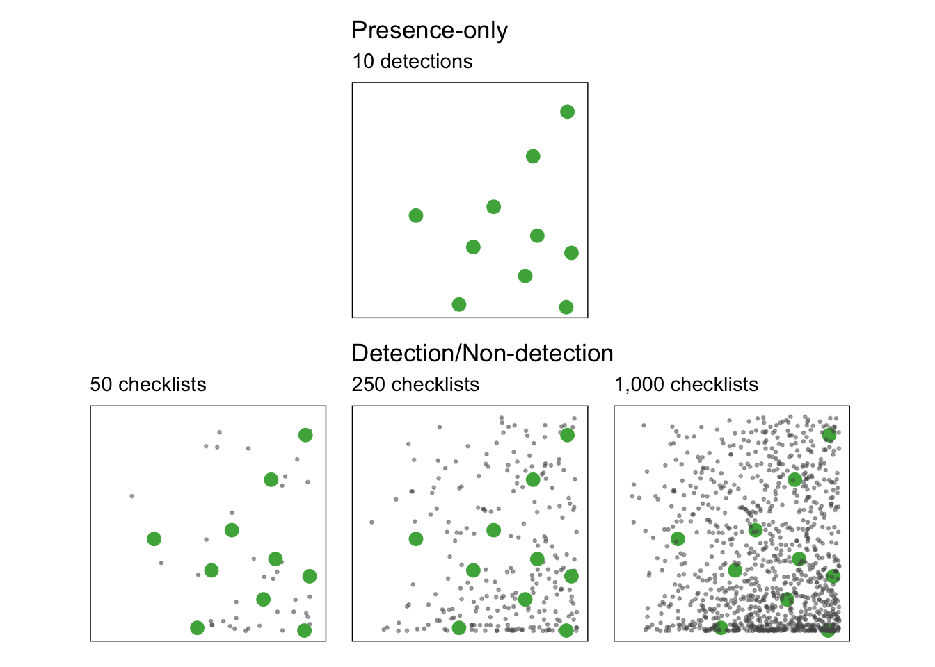
To a large degree, the power of eBird for rigorous analyses comes from the ability to transform the data to produce detection/non-detection data (also referred to as presence/absence data). With presence-only data, but no information of the amount of search effort expended to produce that data, it’s challenging even to estimate how rare or common a species is. For example, consider the 10 detections presented in the top row of the figure below, and ask yourself how common is this species? The bottom row of the figure presents three possible scenarios for the total number of checklists that generated the detections, from left to right
- 50 checklists: in this case the species is fairly common with 20% of checklists reporting the species.
- 250 checklists: in this case the species is uncommon with 4% of checklists reporting the species.
- 1,000 checklists: in this case the species is rare with 1% of checklists reporting the species.
TipTip
Remember that the prevalence of a species on eBird checklists (e.g. 10% of checklists detected a species) is only a relative measure of the actual occupancy probability of that species. To appear on an eBird checklist, a species must occur in an area and be detected by the observer. That detectability always plays a role in determining prevalence and it can vary drastically between regions, seasons, and species.
The EBD alone is a source of presence-only data, with one record for each taxon (typically species) reported. For complete checklists, information about non-detections can be inferred from the SED: if there is a record in the SED but no record for a species in the EBD, then a count of zero individuals of that species can be inferred. This process is referred to a “zero-filling” the data. We can use auk_zerofill() to combine the checklist and observation data together to produce zero-filled, detection/non-detection data.
zf <- auk_zerofill(observations, checklists, collapse = TRUE)By default auk_zerofill() returns a compact representation of the data, consisting of a list of two data frames, one with checklist data and the other with observation data; the use of collapse = TRUE combines these into a single data frame, which will be easier to work with.
Before continuing, we’ll transform some of the variables to a more useful form for modelling. We convert time to a decimal value between 0 and 24, force the distance traveled to 0 for stationary checklists, and create a new variable for speed. Notably, eBirders have the option of entering an “X” rather than a count for a species, to indicate that the species was present, but they didn’t keep track of how many individuals were observed. During the modeling stage, we’ll want the observation_count variable stored as an integer and we’ll convert “X” to NA to allow for this.
# function to convert time observation to hours since midnight
time_to_decimal <- function(x) {
  x <- hms(x, quiet = TRUE)
  hour(x) + minute(x) / 60 + second(x) / 3600
}

# clean up variables
zf <- zf |>
  mutate(
    # convert count to integer and X to NA
    # ignore the warning "NAs introduced by coercion"
    observation_count = as.integer(observation_count),
    # effort_distance_km to 0 for stationary counts
    effort_distance_km = if_else(protocol_type == "Stationary",
                                 0, effort_distance_km),
    # convert duration to hours
    effort_hours = duration_minutes / 60,
    # speed km/h
    effort_speed_kmph = effort_distance_km / effort_hours,
    # convert time to decimal hours since midnight
    hours_of_day = time_to_decimal(time_observations_started),
    # split date into year and day of year
    year = year(observation_date),
    day_of_year = yday(observation_date)
  )
2.7 Accounting for variation in effort
As discussed in the Introduction, variation in effort between checklists makes inference challenging, because it is associated with variation in detectability. When working with semi-structured datasets like eBird, one approach to dealing with this variation is to impose some more consistent structure on the data by filtering observations on the effort variables. This reduces the variation in detectability between checklists. Based on our experience working with these data in the context of eBird Status and Trends, we suggest restricting checklists to traveling or stationary counts less than 6 hours in duration and 10 km in length, at speeds below 100km/h, and with 10 or fewer observers.
# additional filtering
zf_filtered <- zf |>
  filter(protocol_type %in% c("Stationary", "Traveling"),
         effort_hours <= 6,
         effort_distance_km <= 10,
         effort_speed_kmph <= 100,
         number_observers <= 10)
Note that these filtering parameters are based on making predictions at weekly temporal resolution and 3 km spatial resolution. For applications requiring higher spatial precision, stricter filtering on effort_distance_km should be used.
NoteSolution
Let’s pick the checklist duration and make a histogram. The large majority of checklists are well under the 6 hour cutoff, with more than half being less than an hour in duration.
ggplot(zf_filtered) +
  aes(x = effort_hours) +
  geom_histogram(binwidth = 0.5,
                 aes(y = after_stat(count / sum(count)))) +
  scale_y_continuous(limits = c(0, NA), labels = scales::label_percent()) +
  labs(x = "Duration [hours]",
       y = "% of eBird checklists",
       title = "Distribution of eBird checklist duration")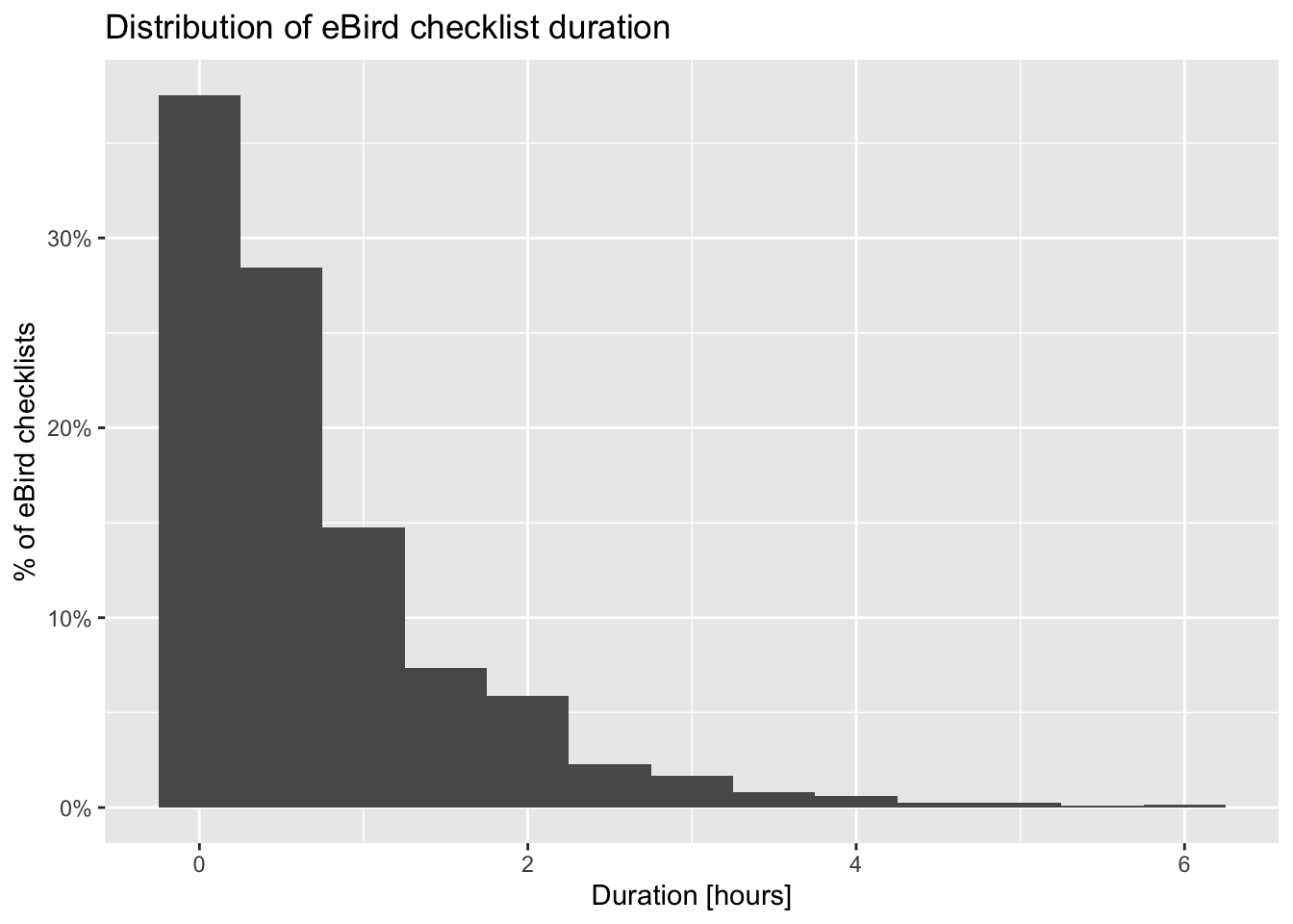
2.7.1 Spatial precision
For each eBird checklists we are provided a single location (longitude/latitude coordinates) specifying where the bird observations occurred. Ideally we want that checklist location to closely match where an observed bird was located. However, there are three main reasons why that may not be the case:
- The bird and observer may not overlap in space. For example, raptors may be observed soaring at a great distance from the observer.
- The checklist location may correspond to an eBird hotspot location rather than the location of the observer. eBird hotspots are public birding locations used to aggregate eBird data, for example, so all checklists at a park or wetland can be grouped together. If observers assign their checklists to an eBird hotspot, the coordinates in the ERD and SED will be those of the hotspot. In some cases, these locations will be a good representation of where the observations occurred, in others they may not be a good representation, for example, if the hotspot location is at the center of a large park but the observations occurred at the edge.
- Traveling checklists survey an area rather than a single point. The amount of area covered will depend on the distance traveled and the compactness of the route taken. For example, a 1 km checklist in a straight line may survey areas further from the checklist coordinates than a 10 km checklist that takes a very circuitous route.
All three of these factors impact the spatial precision of eBird data. Fortunately, many eBird checklists have GPS tracks associated with them. Although these tracks are not available for public use, we can use them to quantify the spatial precision of eBird data. In analyses to inform eBird Status and Trends, we calculated the centroid of all GPS tracks and estimated the distance between that centroid and the reported checklist location. For different maximum checklist distances, we can look at the cumulative distribution of checklists as a function of location error.

As a proxy for checklist compactness, we calculated the minimum radius of a circle fully containing the GPS track of each checklist. Again, we plot the cumulative distribution of this compactness measure for different maximum checklist distances.
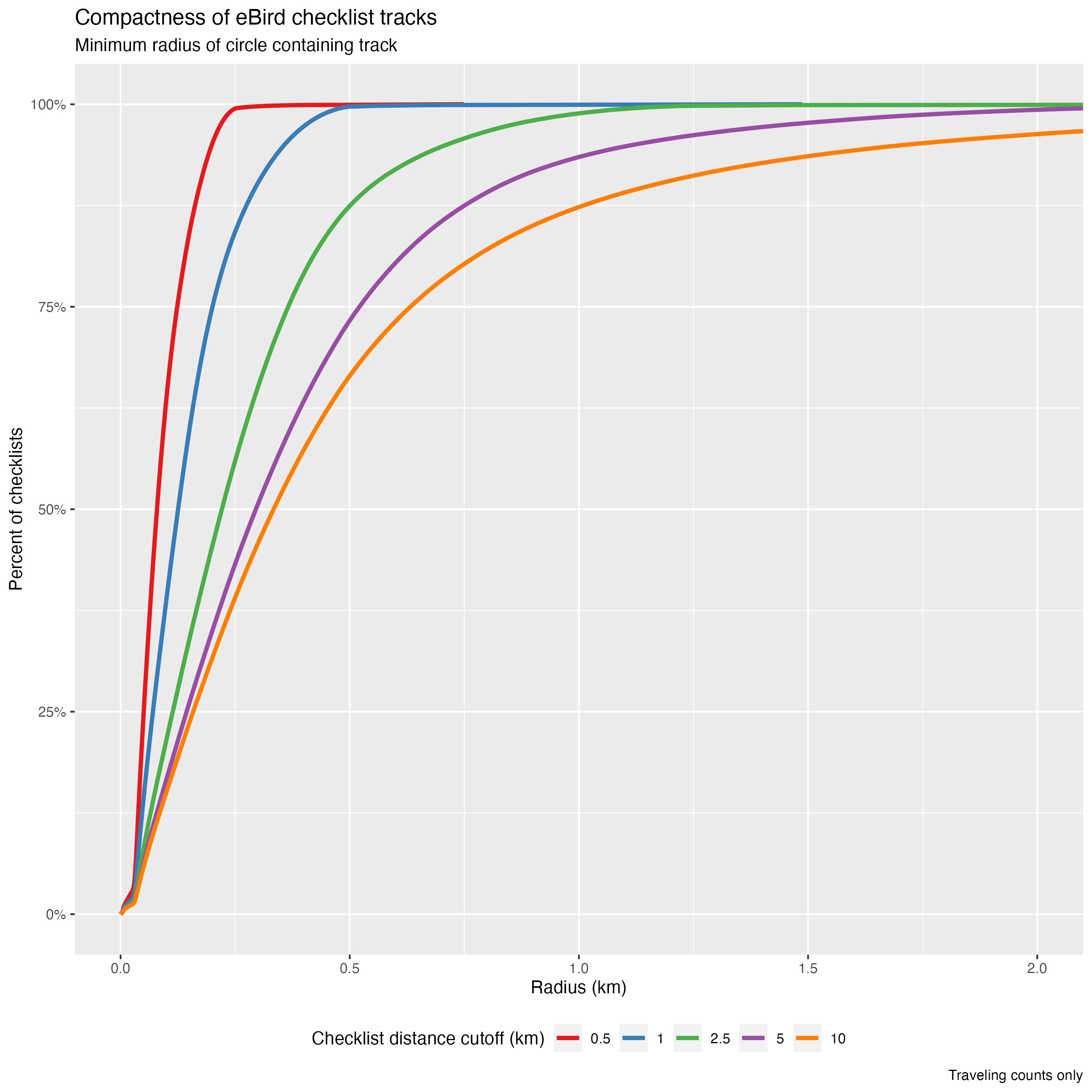
For the specific example of checklists with distances less than 10 km (the cutoff applied above), 94% of traveling checklists are contained within a 1.5 km radius circle and 74% of traveling checklists have location error less than 500 m. This will inform the spatial scale that we use to make predictions in the next chapter. Depending on the precision required for your application, you can use the above plots to adjust the checklist effort filters to control spatial precision.
2.8 Test-train split
For the modeling exercises used in this guide, we’ll hold aside a portion of the data from training to be used as an independent test set to assess the predictive performance of the model. Specifically, we’ll randomly split the data into 80% of checklists for training and 20% for testing. To facilitate this, we create a new variable type that will indicate whether the observation falls in the test set or training set.
zf_filtered$type <- if_else(runif(nrow(zf_filtered)) <= 0.8, "train", "test")
# confirm the proportion in each set is correct
table(zf_filtered$type) / nrow(zf_filtered)
#>
#>  test train
#>   0.2   0.8
Finally, there are a large number of variables in the EBD that are redundant (e.g. both state names and codes are present) or unnecessary for most modeling exercises (e.g. checklist comments and Important Bird Area codes). These can be removed at this point, keeping only the variables we want for modelling. Then we’ll save the resulting zero-filled observations for use in later chapters.
checklists <- zf_filtered |>
  select(checklist_id, observer_id, type,
         observation_count, species_observed,
         state_code, locality_id, latitude, longitude,
         protocol_type, all_species_reported,
         observation_date, year, day_of_year,
         hours_of_day,
         effort_hours, effort_distance_km, effort_speed_kmph,
         number_observers)
write_csv(checklists, "data/checklists-zf_woothr_jun_us-ga.csv", na = "")
If you’d like to ensure you’re using exactly the same data as was used to generate this guide, download the data package mentioned in the setup instructions. Unzip this data package and place the contents in your RStudio project folder.
2.9 Exploratory analysis and visualization
Before proceeding to training species distribution models with these data, it’s worth exploring the dataset to see what we’re working with. Let’s start by making a simple map of the observations. This map uses GIS data available for download in the data package. Unzip this data package and place the contents in your RStudio project folder.
# load gis data
ne_land <- read_sf("data/gis-data.gpkg", "ne_land") |>
  st_geometry()
ne_country_lines <- read_sf("data/gis-data.gpkg", "ne_country_lines") |>
  st_geometry()
ne_state_lines <- read_sf("data/gis-data.gpkg", "ne_state_lines") |>
  st_geometry()
study_region <- read_sf("data/gis-data.gpkg", "ne_states") |>
  filter(state_code == "US-GA") |>
  st_geometry()

# prepare ebird data for mapping
checklists_sf <- checklists |>
  # convert to spatial points
  st_as_sf(coords = c("longitude", "latitude"), crs = 4326) |>
  select(species_observed)

# map
par(mar = c(0.25, 0.25, 4, 0.25))
# set up plot area
plot(st_geometry(checklists_sf),
     main = "Wood Thrush eBird Observations\nJune 2014-2023",
     col = NA, border = NA)
# contextual gis data
plot(ne_land, col = "#cfcfcf", border = "#888888", lwd = 0.5, add = TRUE)
plot(study_region, col = "#e6e6e6", border = NA, add = TRUE)
plot(ne_state_lines, col = "#ffffff", lwd = 0.75, add = TRUE)
plot(ne_country_lines, col = "#ffffff", lwd = 1.5, add = TRUE)
# ebird observations
# not observed
plot(filter(checklists_sf, !species_observed),
     pch = 19, cex = 0.1, col = alpha("#555555", 0.25),
     add = TRUE)
# observed
plot(filter(checklists_sf, species_observed),
     pch = 19, cex = 0.3, col = alpha("#4daf4a", 1),
     add = TRUE)
# legend
legend("bottomright", bty = "n",
       col = c("#555555", "#4daf4a"),
       legend = c("eBird checklist", "Wood Thrush sighting"),
       pch = 19)
box()
In this map, the spatial bias in eBird data becomes immediately obvious, for example, notice the large number of checklists in areas around Atlanta, the largest city in Georgia, in the northern part of the state.
Exploring the effort variables is also a valuable exercise. For each effort variable, we’ll produce both a histogram and a plot of frequency of detection as a function of that effort variable. The histogram will tell us something about birder behavior. For example, what time of day are most people going birding, and for how long? We may also want to note values of the effort variable that have very few observations; predictions made in these regions may be unreliable due to a lack of data. The detection frequency plots tell us how the probability of detecting a species changes with effort.
2.9.1 Time of day
The chance of an observer detecting a bird when present can be highly dependent on time of day. For example, many species exhibit a peak in detection early in the morning during dawn chorus and a secondary peak early in the evening. With this in mind, the first predictor of detection that we’ll explore is the time of day at which a checklist was started. We’ll summarize the data in 1 hour intervals, then plot them. Since estimates of detection frequency are unreliable when only a small number of checklists are available, we’ll only plot hours for which at least 100 checklists are present.
# summarize data by hourly bins
breaks <- seq(0, 24)
labels <- breaks[-length(breaks)] + diff(breaks) / 2
checklists_time <- checklists |>
  mutate(hour_bins = cut(hours_of_day,
                         breaks = breaks,
                         labels = labels,
                         include.lowest = TRUE),
         hour_bins = as.numeric(as.character(hour_bins))) |>
  group_by(hour_bins) |>
  summarise(n_checklists = n(),
            n_detected = sum(species_observed),
            det_freq = mean(species_observed))

# histogram
g_tod_hist <- ggplot(checklists_time) +
  aes(x = hour_bins, y = n_checklists) +
  geom_segment(aes(xend = hour_bins, y = 0, yend = n_checklists),
               color = "grey50") +
  geom_point() +
  scale_x_continuous(breaks = seq(0, 24, by = 3), limits = c(0, 24)) +
  scale_y_continuous(labels = scales::comma) +
  labs(x = "Hours since midnight",
       y = "# checklists",
       title = "Distribution of observation start times")

# frequency of detection
g_tod_freq <- ggplot(checklists_time |> filter(n_checklists > 100)) +
  aes(x = hour_bins, y = det_freq) +
  geom_line() +
  geom_point() +
  scale_x_continuous(breaks = seq(0, 24, by = 3), limits = c(0, 24)) +
  scale_y_continuous(labels = scales::percent) +
  labs(x = "Hours since midnight",
       y = "% checklists with detections",
       title = "Detection frequency")

# combine
grid.arrange(g_tod_hist, g_tod_freq)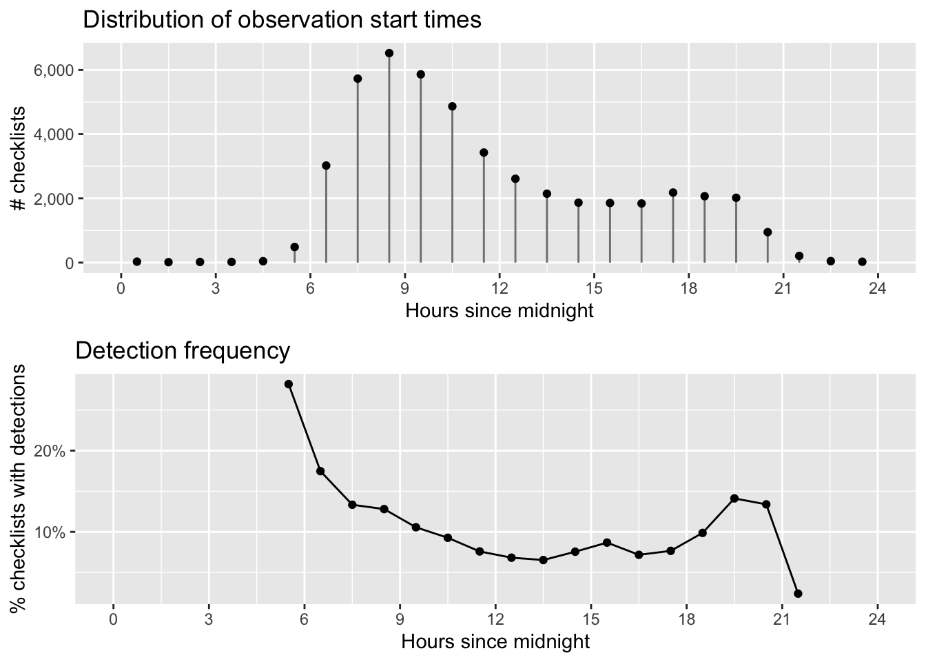
As expected, Wood Thrush detectability is highest early in the morning and quickly falls off as the day progresses. In later chapters, we’ll make predictions at the peak time of day for detectability to limit the effect of this variation. The majority of checklist submissions also occurs in the morning; however, there are reasonable numbers of checklists between 6am and 9pm. It’s in this region that our model estimates will be most reliable.
2.9.2 Checklist duration
When we filtered the eBird data in Section 2.7, we restricted observations to those from checklists 6 hours in duration or shorter to reduce variability. Let’s see what sort of variation remains in checklist duration.
# summarize data by hour long bins
breaks <- seq(0, 6)
labels <- breaks[-length(breaks)] + diff(breaks) / 2
checklists_duration <- checklists |>
  mutate(duration_bins = cut(effort_hours,
                             breaks = breaks,
                             labels = labels,
                             include.lowest = TRUE),
         duration_bins = as.numeric(as.character(duration_bins))) |>
  group_by(duration_bins) |>
  summarise(n_checklists = n(),
            n_detected = sum(species_observed),
            det_freq = mean(species_observed))

# histogram
g_duration_hist <- ggplot(checklists_duration) +
  aes(x = duration_bins, y = n_checklists) +
  geom_segment(aes(xend = duration_bins, y = 0, yend = n_checklists),
               color = "grey50") +
  geom_point() +
  scale_x_continuous(breaks = breaks) +
  scale_y_continuous(labels = scales::comma) +
  labs(x = "Checklist duration [hours]",
       y = "# checklists",
       title = "Distribution of checklist durations")

# frequency of detection
g_duration_freq <- ggplot(checklists_duration |> filter(n_checklists > 100)) +
  aes(x = duration_bins, y = det_freq) +
  geom_line() +
  geom_point() +
  scale_x_continuous(breaks = breaks) +
  scale_y_continuous(labels = scales::percent) +
  labs(x = "Checklist duration [hours]",
       y = "% checklists with detections",
       title = "Detection frequency")

# combine
grid.arrange(g_duration_hist, g_duration_freq)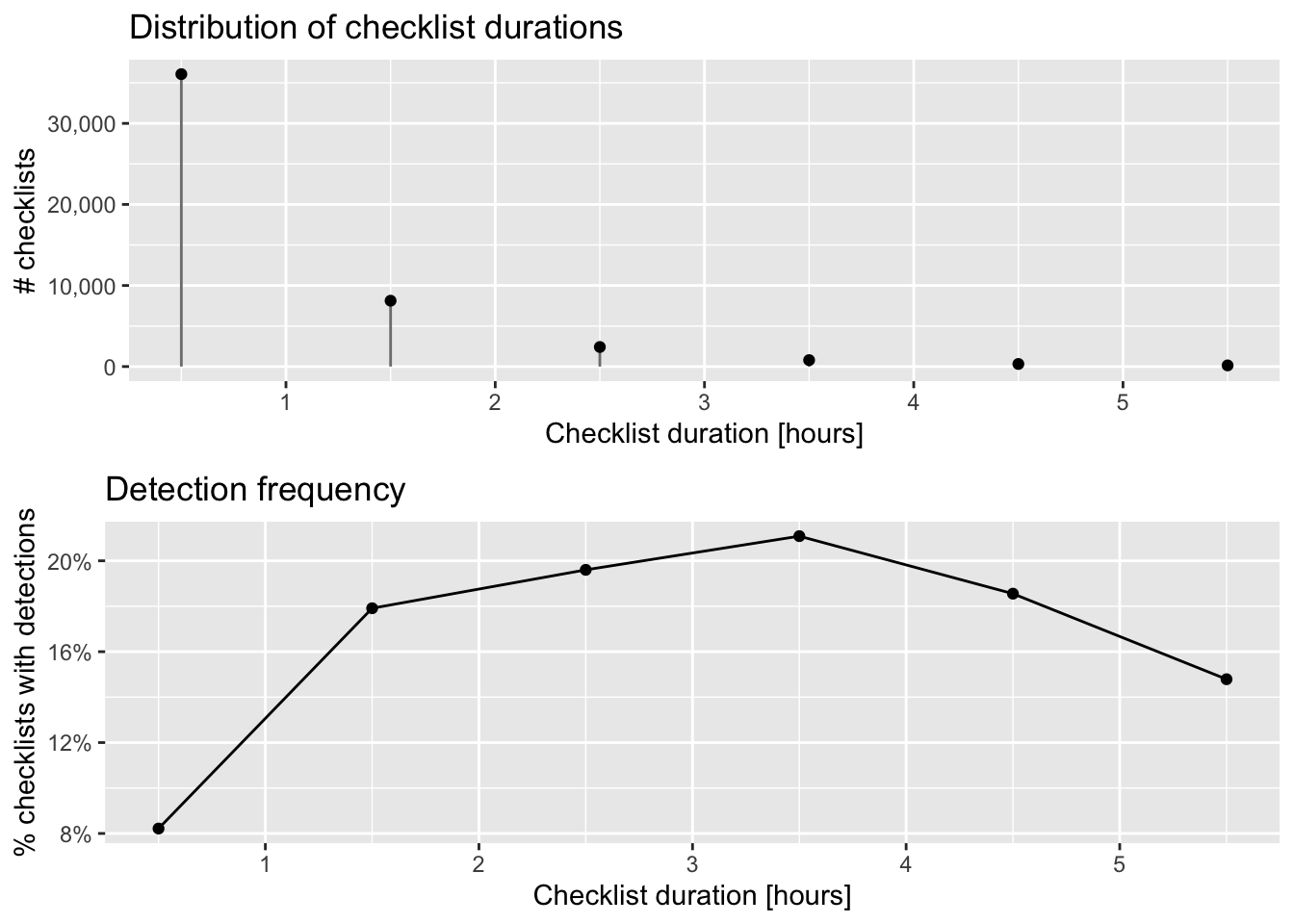
The majority of checklists are an hour or shorter and there is a rapid decline in the frequency of checklists with increasing duration. In addition, longer searches yield a higher chance of detecting a Wood Thrush. In many cases, there is a saturation effect, with searches beyond a given length producing little additional benefit; however, here there appears to be a drop off in detection for checklists longer than 3.5 hours.
2.9.3 Distance traveled
As with checklist duration, we expect a priori that the greater the distance someone travels, the greater the probability of encountering at least one Wood Thrush. Let’s see if this expectation is met. Note that we have already truncated the data to checklists less than 10 km in length.
# summarize data by 1 km bins
breaks <- seq(0, 10)
labels <- breaks[-length(breaks)] + diff(breaks) / 2
checklists_dist <- checklists |>
  mutate(dist_bins = cut(effort_distance_km,
                         breaks = breaks,
                         labels = labels,
                         include.lowest = TRUE),
         dist_bins = as.numeric(as.character(dist_bins))) |>
  group_by(dist_bins) |>
  summarise(n_checklists = n(),
            n_detected = sum(species_observed),
            det_freq = mean(species_observed))

# histogram
g_dist_hist <- ggplot(checklists_dist) +
  aes(x = dist_bins, y = n_checklists) +
  geom_segment(aes(xend = dist_bins, y = 0, yend = n_checklists),
               color = "grey50") +
  geom_point() +
  scale_x_continuous(breaks = breaks) +
  scale_y_continuous(labels = scales::comma) +
  labs(x = "Distance travelled [km]",
       y = "# checklists",
       title = "Distribution of distance travelled")

# frequency of detection
g_dist_freq <- ggplot(checklists_dist |> filter(n_checklists > 100)) +
  aes(x = dist_bins, y = det_freq) +
  geom_line() +
  geom_point() +
  scale_x_continuous(breaks = breaks) +
  scale_y_continuous(labels = scales::percent) +
  labs(x = "Distance travelled [km]",
       y = "% checklists with detections",
       title = "Detection frequency")

# combine
grid.arrange(g_dist_hist, g_dist_freq)
As with duration, the majority of observations are from short checklists (less than half a kilometer). One fortunate consequence of this is that most checklists will be contained within a small area within which habitat is not likely to show high variability. In Chapter 3, we will summarize land cover data within circles 3 km in diameter, centered on each checklist, and it appears that the vast majority of checklists will stay contained within this area.
2.9.4 Number of observers
Finally, let’s consider the number of observers whose observation are being reported in each checklist. We expect that at least up to some number of observers, reporting rates will increase; however, in working with these data we have found cases of declining detection rates for very large groups. With this in mind we have already restricted checklists to those with 10 or fewer observers, thus removing the very largest groups (prior to filtering, some checklists had as many as 180 observers!).
# summarize data
breaks <- seq(0, 10)
labels <- seq(1, 10)
checklists_obs <- checklists |>
  mutate(obs_bins = cut(number_observers,
                        breaks = breaks,
                        label = labels,
                        include.lowest = TRUE),
         obs_bins = as.numeric(as.character(obs_bins))) |>
  group_by(obs_bins) |>
  summarise(n_checklists = n(),
            n_detected = sum(species_observed),
            det_freq = mean(species_observed))

# histogram
g_obs_hist <- ggplot(checklists_obs) +
  aes(x = obs_bins, y = n_checklists) +
  geom_segment(aes(xend = obs_bins, y = 0, yend = n_checklists),
               color = "grey50") +
  geom_point() +
  scale_x_continuous(breaks = breaks) +
  scale_y_continuous(labels = scales::comma) +
  labs(x = "# observers",
       y = "# checklists",
       title = "Distribution of the number of observers")

# frequency of detection
g_obs_freq <- ggplot(checklists_obs |> filter(n_checklists > 100)) +
  aes(x = obs_bins, y = det_freq) +
  geom_line() +
  geom_point() +
  scale_x_continuous(breaks = breaks) +
  scale_y_continuous(labels = scales::percent) +
  labs(x = "# observers",
       y = "% checklists with detections",
       title = "Detection frequency")

# combine
grid.arrange(g_obs_hist, g_obs_freq)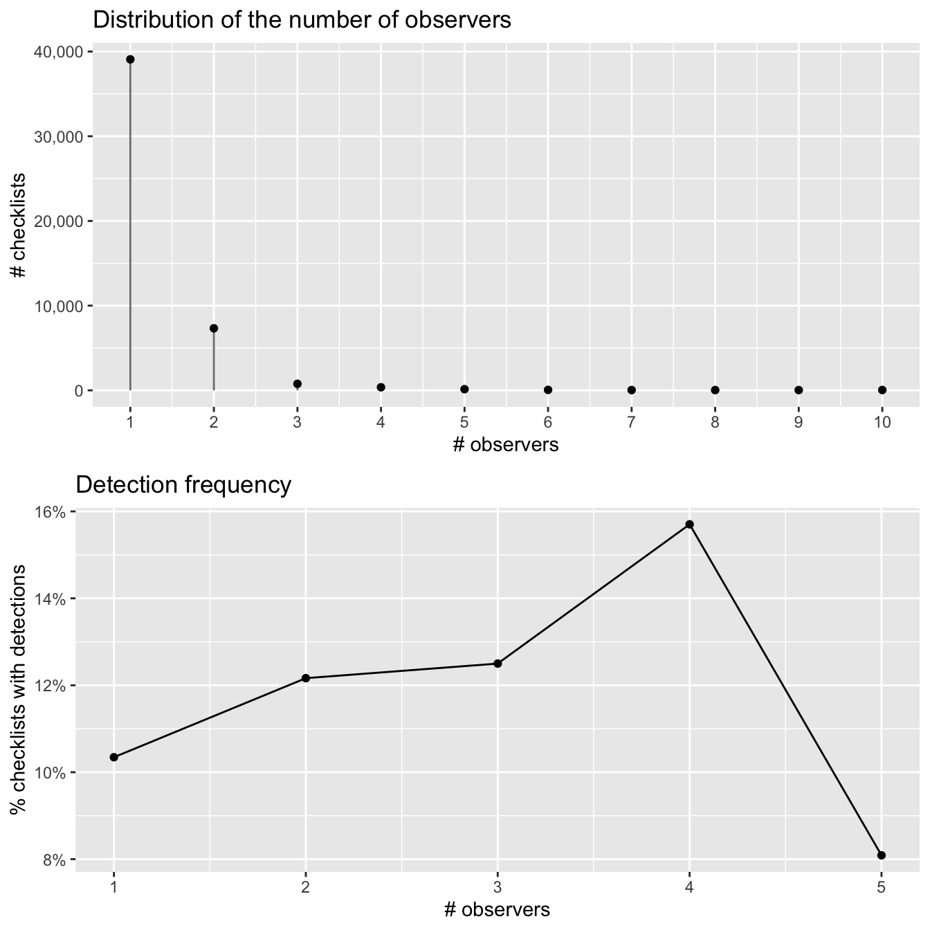
The majority of checklists have one or two observers and there appears to be an increase in detection frequency with more observers. However, it’s hard to distinguish a discernible pattern in the noise here, likely because there are so few checklists with more than 3 observers.